Speech to Speech Foundation Models

Over the past few years, conversational AI has been progressing at a pace that few of us could have predicted. Voice assistants no longer sound robotic, realtime translation systems can preserve the emotional nuances of a speaker’s voice, and voice cloning requires only a handful of seconds of reference audio. At the heart of many of these advances lies a class of models collectively known as Speech to Speech (S2S) systems, a technology that is rapidly transforming the way we communicate across languages, platforms, and modalities.

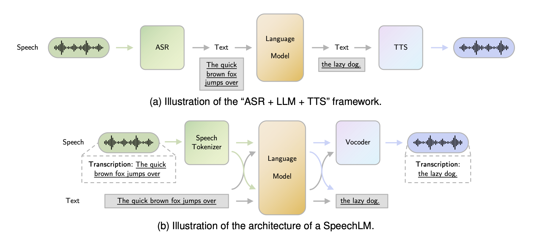
Figure 1 : The paradigm shift in speech AI: (a) traditional cascaded ASR + LLM + TTS pipeline versus (b) end to end Speech Language Models that process and generate speech directly, preserving paralinguistic information such as pitch, timbre, and emotion. Figure from Cui et al.^[12]

Unlike traditional pipelines that chain automatic speech recognition (ASR), natural language processing (NLP), and text to speech (TTS) as discrete sequential stages, modern S2S models learn to map acoustic features directly from source to target, preserving the richness of spoken communication that text mediated pipelines inevitably discard. These models power realtime voice assistants, simultaneous translation, and voice conversion applications. The implications are significant: a Mandarin speaker can converse naturally with an English speaker in near realtime, a content creator can dub their videos in dozens of languages with their own voice, and assistants can respond with expressive, human like speech that captures emotion and intent.

The journey from autoregressive WaveNet based approaches to parallel, flow based, and now diffusion based architectures has dramatically reduced latency while improving naturalness. For folks building production systems, understanding the mathematical foundations, architectural choices, and inference optimization techniques is essential. In this post, we will walk through the high-level architecture of modern S2S systems, explore the mathematical foundations behind each component, build a simplified S2S pipeline in PyTorch, and close with predictions on where this technology is heading.

High Level Architecture

A modern S2S system can be decomposed into four tightly coupled stages. It begins with speech analysis, where acoustic features are extracted from the source speaker’s audio. The content encoding stage then isolates the linguistic content (what was being said) from the speaker identity (who said it). Speaker conditioning applies the target speaker’s characteristics through learned embeddings or conditioning signals, and finally, waveform synthesis generates natural sounding audio in the target speaker’s voice.

At a high level, the pipeline looks something like this:

Source Speech Audio
    ↓
[STFT/Mel-Spectrogram Extraction]
    ↓
[Content Encoder] → Phonetic Posteriorgrams (PPGs) or latent representation
    ↓
[Speaker Encoder] → Target speaker embedding from reference utterance
    ↓
[Acoustic Model] → Target speaker's mel-spectrogram
    ↓
[Neural Vocoder (HiFi-GAN/WaveRNN)] → Target waveform
    ↓
Output Speech Audio

Let’s walk through each component in detail.

1. Acoustic Encoder

The acoustic encoder’s primary role is to extract speaker invariant linguistic content from the source speech signal while discarding speaker specific characteristics. This component operates on acoustic features such as mel-spectrograms (typically 80-128 frequency bins) computed from 16 kHz or higher sample rate audio, with frame shifts of 10-12.5 ms. Modern implementations employ dilated or causal convolutional layers (commonly 3-5 layers with 256-512 hidden units) to capture temporal dependencies across a receptive field of 100-400 ms, or recurrent architectures (BiLSTM/GRU) with 128-512 hidden dimensions for bidirectional context modeling. The encoder produces frame level representations either as Phonetic Posteriorgrams (PPGs) from auxiliary phoneme classifiers, learned latent vectors, or bottleneck features typically dimensioned at 64-256 dimensions per frame. These representations aim to capture phonetic content while being invariant to speaker identity, though perfect speaker-content disentanglement remains an open challenge requiring careful training objectives (e.g., adversarial speaker loss, information bottleneck constraints).

2. Speaker Encoder

The speaker encoder’s objective is to produce a fixed dimensional embedding that captures the unique voice characteristics and timbre of a speaker while remaining invariant to linguistic content. This component processes either the reference utterance from the target speaker or, in some architectures, extracts speaker information from the source audio itself. The most common implementation leverages bidirectional LSTM networks (typically 2-3 layers with 256-768 hidden units) that process frame level acoustic features across the entire utterance, followed by a temporal pooling mechanism either mean/max pooling across the time dimension or an attention based aggregation to collapse the variable length sequence into a fixed size representation. The resulting speaker embedding is typically a dense vector of ~256 to 512 dimensions that encodes speaker specific attributes such as pitch range, vocal tract characteristics, and speaking rate. Training often employs metric learning objectives like triplet loss or generalized end to end (GE2E) loss to ensure that embeddings from the same speaker cluster tightly in the latent space while maintaining separation from other speakers, enabling effective few shot or zero shot voice cloning capabilities.

3. Acoustic Model/Decoder

The acoustic model, often referred to as the decoder, serves as the synthesis engine that transforms the disentangled content representation and target speaker embedding into acoustic features that characterize the target speaker’s voice. This component performs the critical task of fusing linguistic content from the content encoder with speaker characteristics from the speaker encoder to generate mel-spectrograms, typically 80 to 128 dimensional feature vectors computed over overlapping time frames with 10 to 12.5 ms shifts. The architectural landscape here divides into two paradigms: autoregressive models (such as Tacotron 2 or Transformer-TTS variants) that generate acoustic frames sequentially, conditioning each step on previously generated frames through recurrent connections or causal attention masks, and non-autoregressive models (like FastSpeech 2, VITS, or parallel WaveGAN variants) that predict all frames simultaneously through learned duration models or alignment mechanisms. Autoregressive architectures, while often producing higher quality outputs with better prosody modeling, suffer from quadratic complexity and sequential dependencies that limit parallelization and increase latency (typically 100-500 ms RTF on GPU). Non-autoregressive approaches sacrifice some prosodic naturalness for massive speedups (often 10-100x faster, achieving RTFs of 0.01-0.05), making them preferable for realtime applications. The decoder typically employs attention mechanisms (location-sensitive, monotonic, or alignment-free techniques using learned duration predictors) to establish correspondence between content representations and output frames. The output mel-spectrogram serves as an intermediate representation that captures the spectral envelope, formant structure, and temporal dynamics of the target speech while remaining tractable for neural vocoder processing.

4. Neural Vocoder

The neural vocoder represents the final synthesis stage, responsible for converting mel-spectrograms (compressed acoustic representations) back into high-fidelity raw waveforms at the target sample rate (typically 22.05 kHz or 24 kHz). This task, often termed vocoding or waveform generation, requires modeling the complex conditional distribution over 16-bit or 24-bit audio samples while capturing spectral details and temporal coherence. The vocoder architecture landscape encompasses three primary paradigms: autoregressive models like WaveNet employ dilated causal convolutions to factorize the joint distribution into a product of conditionals, achieving exceptional audio quality (MOS scores often >4.3) but suffering severe latency penalties (typically 100-1000 ms RTF) due to sequential sample generation; generative adversarial approaches such as HiFi-GAN leverage multiple discriminators (scale and multi period) operating on progressively upsampled feature maps with transpose convolutions, achieving realtime synthesis (RTF <0.01) with competitive quality (MOS >4.0) through adversarial training that captures perceptually important characteristics; and flow based models like WaveGlow utilize invertible transformations (affine coupling layers) to map Gaussian noise through learned bijections conditioned on mel-spectrograms, offering deterministic, differentiable synthesis with RTFs of 0.05-0.1 and improved stability compared to GANs. For production S2S systems, HiFi-GAN has become the de facto standard due to its superior speed and quality tradeoff, though emerging diffusion based vocoders are beginning to challenge this dominance by offering comparable quality with enhanced robustness to out of distribution mel-spectrogram inputs and improved generalization across diverse speakers and acoustic conditions.

Mathematical Foundation

Now that we’ve looked at the high level architecture, let’s jump into the mathematical foundation to understand these systems in detail. The elegance of S2S systems lies in how classical signal processing theory interfaces with modern deep learning each component we discussed above has precise mathematical underpinnings that govern its behavior and the architectural decisions.

1. Short-Time Fourier Transform (STFT) and Mel-Spectrograms

The foundation of acoustic feature extraction rests firmly on signal processing principles. Raw audio waveforms, while containing all necessary information, are unwieldy for neural networks to process directly. The Short-Time Fourier Transform provides a time-frequency representation that decomposes the signal into its constituent frequencies at each point in time, enabling networks to reason about spectral content evolution^[1]. The STFT applies the discrete Fourier transform to overlapping windowed segments of the input signal:

Here,

• $x(n)$ represents the input audio signal
• $w(n)$ is a window function (typically Hamming or Hann windows that taper smoothly to zero at the edges to reduce spectral leakage)
• $m$ indexes the frame
• $k$ indexes the frequency bin
• $H$ denotes the hop length (typically 128 samples at 16kHz, corresponding to 8ms)
• $N$ is the FFT size (typically 512 or 1024 samples)

The choice of these hyperparameters represents a fundamental tradeoff: larger FFT sizes provide finer frequency resolution but coarser temporal resolution, while the hop length determines the overlap between adjacent frames and thus the temporal granularity of the representation.

However, raw spectrograms contain more frequency resolution than human perception requires, and crucially, human auditory perception is approximately logarithmic in frequency we perceive the interval between 100 Hz and 200 Hz as similar to the interval between 1000 Hz and 2000 Hz. The mel scale, derived from psychoacoustic experiments, captures this non-linear relationship:

The mel-spectrogram applies triangular filterbanks spaced uniformly on the mel scale to the power spectrum, then takes the logarithm to compress dynamic range and better match human loudness perception:

In this formulation, $H_b(k)$ represents the triangular mel filterbank for bin $b$ (typically 80 filters spanning frequencies from roughly 0 to 8000 Hz), and $\alpha$ is a scaling constant that ensures numerical stability by preventing log(0). This 80 dimensional representation at each time frame serves as the primary input to most S2S system components, striking a balance between compact representation and sufficient information for high quality reconstruction.

2. Sequence to Sequence Mapping with Attention

The encoder decoder architecture with attention forms the backbone of how S2S systems align and transform representations between source and target domains. The attention mechanism allows the decoder to dynamically focus on relevant parts of the encoded source sequence when generating each output frame, rather than compressing the entire input into a fixed-length bottleneck. For a deeper dive into attention mechanisms and their optimization techniques, see my detailed exploration in Key-Value Caching in Large Language Models. The scaled dot product attention^[2] computes alignment weights between query vectors and key vectors, then uses these weights to compute a weighted sum of value vectors:

The scaling factor $\sqrt{d_k}$ (where $d_k$ is the key dimension) prevents the dot products from growing too large in magnitude as the dimensionality increases, which would push the softmax into regions of extremely small gradients.

Modern S2S systems employ multi head attention, which allows the model to jointly attend to information from different representation subspaces at different positions:

$ where \ \text{head}_i = \text{Attention}(QW_i^Q, KW_i^K, VW_i^V) $

Each head learns different attention patterns some might focus on local acoustic context, others on longer range prosodic dependencies and the concatenated outputs are linearly projected to produce the final attended representation.

3. Duration Prediction and Alignment

This is a very interesting segment. Non autoregressive models achieve their speed advantage by predicting all output frames simultaneously, but this requires explicitly modeling the alignment between input (phoneme/content) and output (acoustic frame) sequences. Duration prediction modules learn to estimate how many acoustic frames each input token should span. The duration loss is typically formulated in log-space to handle the wide dynamic range of phoneme durations (from tens of milliseconds for plosives to hundreds for sustained vowels):

Here, $d_i$ represents the ground truth duration of phoneme $i$ (extracted via forced alignment or learned jointly), and $\hat{d}_i$ is the predicted duration. The addition of 1 before taking the logarithm prevents numerical issues when durations are zero (which can occur for deleted phonemes in fast speech) and provides a form of Laplace smoothing. During inference, predicted durations are used to expand the content representation to match the target acoustic sequence length.

4. Speaker Embedding Learning

The speaker encoder must learn a representation space where embeddings from the same speaker cluster together while embeddings from different speakers remain well separated. This is fundamentally a metric learning problem, and the Generalized End to End (GE2E) framework^[3] demonstrates that contrastive losses provide an effective training objective:

This InfoNCE style loss maximizes the cosine similarity $\text{sim}(s_1, s_2)$ between embeddings from the same speaker (positive pairs) while minimizing similarity to embeddings from other speakers in the batch (negative samples). The temperature parameter $\tau$ controls the sharpness of the distribution. Lower temperatures create harder contrasts that push the model to learn more discriminative features, while higher temperatures provide softer gradients that can aid early training stability. This formulation enables fewshot and zeroshot voice cloning: at inference time, a brief reference utterance from a new speaker is encoded, and the resulting embedding conditions the decoder to synthesize speech in that speaker’s voice.

5. Vocoder Loss Functions

Neural vocoders face the challenging task of generating high-fidelity audio waveforms from mel-spectrogram inputs, and their training objectives must capture both spectral accuracy and perceptual quality. The reconstruction loss combines L1 and L2 terms computed on spectrograms at multiple resolutions to ensure both sharp spectral details and overall envelope matching:

The L1 loss encourages sparse, sharp spectral predictions while the L2 loss penalizes large deviations more heavily; the weighting $\alpha$ balances these complementary objectives.

GAN based vocoders like HiFi-GAN^[4] add adversarial losses using a least squares formulation that push the generator to produce waveforms indistinguishable from real audio to a learned discriminator:

Here $D$ is the discriminator network, $x$ represents real audio samples, and $\hat{x}$ represents generated audio. The generator in turn minimizes $\mathbb{E}[(D(\hat{x}) - 1)^2]$, pushing its outputs to be classified as real. HiFi-GAN employs multiple discriminators operating at different scales and periodicities to capture both waveform details and longer range structure.

The feature matching loss provides additional supervisory signal by encouraging the generator to produce waveforms whose intermediate discriminator activations match those of real audio:

Here $D^l$ extracts features from layer $l$ of the discriminator, and $N_l$ is the number of features in that layer. This loss stabilizes GAN training by providing dense gradient signal from multiple levels of the discriminator’s learned feature hierarchy, rather than relying solely on the scalar adversarial signal.

Implementation: Building a Dummy S2S Pipeline

With the mathematical foundations in place, let us build a simplified S2S pipeline in PyTorch. The goal here is pedagogical clarity rather than production readiness. Each module maps directly to one of the architectural components discussed above, and the code is intentionally compact so we can follow every data transformation from input waveform to output speech. We will implement five core modules: a mel-spectrogram extractor that converts raw audio to time frequency representations, a content encoder that extracts speaker invariant linguistic features, a speaker encoder that produces fixed dimensional voice embeddings, an acoustic decoder that fuses content and speaker identity to generate target mel-spectrograms, and a simplified vocoder that converts mel-spectrograms back into waveforms.

Mel-Spectrogram Extractor

The first step in any S2S pipeline is converting raw audio into mel-spectrograms. This module implements the STFT and mel filterbank application we derived in the mathematical foundation section. The _create_mel_filterbank method constructs triangular filters spaced uniformly on the mel scale, and the forward pass computes the power spectrum via STFT, applies the filterbank, and takes the logarithm for dynamic range compression.

import torch
import torch.nn as nn
import torch.nn.functional as F
import numpy as np

class MelSpectrogramExtractor(nn.Module):
    """Extracts mel-spectrograms from raw audio waveforms."""
    def __init__(self, sample_rate=16000, n_fft=1024, hop_length=256, 
                 n_mels=80, f_min=0, f_max=8000):
        super().__init__()
        self.n_fft = n_fft
        self.hop_length = hop_length
        
        mel_fb = self._create_mel_filterbank(sample_rate, n_fft, n_mels, f_min, f_max)
        self.register_buffer('mel_fb', mel_fb)
        self.register_buffer('window', torch.hann_window(n_fft))
    
    def _create_mel_filterbank(self, sr, n_fft, n_mels, f_min, f_max):
        """Create triangular mel filterbank matrix."""
        mel_min = 2595 * np.log10(1 + f_min / 700)
        mel_max = 2595 * np.log10(1 + f_max / 700)
        mel_points = np.linspace(mel_min, mel_max, n_mels + 2)
        hz_points = 700 * (10 ** (mel_points / 2595) - 1)
        bin_points = np.floor((n_fft + 1) * hz_points / sr).astype(int)
        
        filterbank = np.zeros((n_mels, n_fft // 2 + 1))
        for i in range(n_mels):
            for j in range(bin_points[i], bin_points[i + 1]):
                filterbank[i, j] = (j - bin_points[i]) / (bin_points[i + 1] - bin_points[i])
            for j in range(bin_points[i + 1], bin_points[i + 2]):
                filterbank[i, j] = (bin_points[i + 2] - j) / (bin_points[i + 2] - bin_points[i + 1])
        
        return torch.FloatTensor(filterbank)
    
    def forward(self, waveform):
        """
        Args:
            waveform: [batch_size, num_samples]
        Returns:
            mel_spec: [batch_size, n_mels, time_frames]
        """
        stft = torch.stft(waveform, self.n_fft, self.hop_length,
                          window=self.window, return_complex=True)
        power_spec = torch.abs(stft) ** 2
        mel_spec = torch.matmul(self.mel_fb, power_spec)
        return torch.log(mel_spec + 1e-9)

Content Encoder

The content encoder uses convolutional layers for local feature extraction followed by a bidirectional LSTM for temporal modeling. Notice how the architecture mirrors the mathematical formulation: convolutions capture local spectral patterns (analogous to the windowed analysis in STFT), while the LSTM models sequential dependencies across frames. The bidirectional output is projected down to the content dimension to produce a compact, speaker invariant representation at each time step.

class ContentEncoder(nn.Module):
    """Extracts speaker invariant linguistic content from mel-spectrograms."""
    def __init__(self, n_mels=80, hidden_dim=256, content_dim=128):
        super().__init__()
        self.conv_layers = nn.Sequential(
            nn.Conv1d(n_mels, hidden_dim, kernel_size=5, padding=2),
            nn.BatchNorm1d(hidden_dim),
            nn.ReLU(),
            nn.Conv1d(hidden_dim, hidden_dim, kernel_size=5, padding=2),
            nn.BatchNorm1d(hidden_dim),
            nn.ReLU(),
            nn.Conv1d(hidden_dim, hidden_dim, kernel_size=5, padding=2),
            nn.BatchNorm1d(hidden_dim),
            nn.ReLU(),
        )
        self.lstm = nn.LSTM(hidden_dim, content_dim, num_layers=2,
                            batch_first=True, bidirectional=True)
        self.projection = nn.Linear(content_dim * 2, content_dim)
    
    def forward(self, mel_spec):
        """
        Args:
            mel_spec: [batch_size, n_mels, time_frames]
        Returns:
            content: [batch_size, time_frames, content_dim]
        """
        x = self.conv_layers(mel_spec)        # [batch, hidden, time]
        x = x.transpose(1, 2)                 # [batch, time, hidden]
        x, _ = self.lstm(x)                   # [batch, time, 2*content_dim]
        return self.projection(x)             # [batch, time, content_dim]

Speaker Encoder

The speaker encoder processes a reference utterance and collapses it into a single embedding vector through temporal average pooling, followed by L2 normalization. This is the component trained with the contrastive loss $\mathcal{L}_{speaker}$ described earlier. The L2 normalization ensures that speaker similarity can be measured via cosine distance in the embedding space, which is critical for the few shot voice cloning capability.

class SpeakerEncoder(nn.Module):
    """Produces fixed dimensional speaker embeddings from reference utterances."""
    def __init__(self, n_mels=80, hidden_dim=256, embedding_dim=256):
        super().__init__()
        self.lstm = nn.LSTM(n_mels, hidden_dim, num_layers=3,
                            batch_first=True, bidirectional=True)
        self.projection = nn.Linear(hidden_dim * 2, embedding_dim)
    
    def forward(self, mel_spec):
        """
        Args:
            mel_spec: [batch_size, n_mels, time_frames]
        Returns:
            embedding: [batch_size, embedding_dim]
        """
        x = mel_spec.transpose(1, 2)          # [batch, time, n_mels]
        x, _ = self.lstm(x)                   # [batch, time, 2*hidden]
        embedding = x.mean(dim=1)             # temporal average pooling
        embedding = self.projection(embedding)
        return F.normalize(embedding, p=2, dim=-1)

Acoustic Decoder

The decoder fuses content representations with the speaker embedding by projecting the speaker vector into a higher dimensional space and concatenating it with content features at every time step. The LSTM then generates target mel-spectrogram frames conditioned on both streams. This concatenation based conditioning is the simplest approach; production systems often use more sophisticated techniques like FiLM (Feature-wise Linear Modulation) or cross-attention for tighter integration.

class AcousticDecoder(nn.Module):
    """Generates target mel-spectrograms from content + speaker embedding."""
    def __init__(self, content_dim=128, speaker_dim=256,
                 hidden_dim=512, n_mels=80):
        super().__init__()
        self.speaker_proj = nn.Linear(speaker_dim, hidden_dim)
        self.decoder_lstm = nn.LSTM(content_dim + hidden_dim, hidden_dim,
                                     num_layers=2, batch_first=True)
        self.mel_proj = nn.Linear(hidden_dim, n_mels)
    
    def forward(self, content, speaker_embedding):
        """
        Args:
            content: [batch_size, time_frames, content_dim]
            speaker_embedding: [batch_size, speaker_dim]
        Returns:
            mel_output: [batch_size, n_mels, time_frames]
        """
        batch_size, time_frames, _ = content.shape
        spk = self.speaker_proj(speaker_embedding)           # [batch, hidden]
        spk = spk.unsqueeze(1).expand(-1, time_frames, -1)  # [batch, time, hidden]
        x = torch.cat([content, spk], dim=-1)
        x, _ = self.decoder_lstm(x)
        return self.mel_proj(x).transpose(1, 2)  # [batch, n_mels, time]

Simplified Vocoder

Our vocoder uses a stack of transposed convolutions to progressively upsample mel frames back to waveform resolution. This is a stripped-down version of the HiFi-GAN generator architecture^[4], omitting the multi receptive field fusion and multi scale discriminators for simplicity. The upsample rates (8, 8, 2, 2) multiply to 256, which matches our hop length of 256, so the output waveform has approximately the same number of samples as the input audio.

class SimpleVocoder(nn.Module):
    """Converts mel-spectrograms to waveforms via transposed convolutions."""
    def __init__(self, n_mels=80, upsample_rates=[8, 8, 2, 2],
                 hidden_dim=256):
        super().__init__()
        self.input_conv = nn.Conv1d(n_mels, hidden_dim, kernel_size=7, padding=3)
        
        layers = []
        in_ch = hidden_dim
        for rate in upsample_rates:
            out_ch = in_ch // 2
            layers.append(nn.ConvTranspose1d(
                in_ch, out_ch, kernel_size=rate * 2,
                stride=rate, padding=rate // 2))
            layers.append(nn.LeakyReLU(0.1))
            in_ch = out_ch
        
        self.upsample = nn.Sequential(*layers)
        self.output_conv = nn.Conv1d(in_ch, 1, kernel_size=7, padding=3)
        self.tanh = nn.Tanh()
    
    def forward(self, mel_spec):
        """
        Args:
            mel_spec: [batch_size, n_mels, time_frames]
        Returns:
            waveform: [batch_size, 1, num_samples]
        """
        x = self.input_conv(mel_spec)
        x = self.upsample(x)
        return self.tanh(self.output_conv(x))

Tying It All Together

The full pipeline chains each module in the order we described in the architecture section. Source audio is analyzed for content, reference audio provides the speaker identity, and the decoder fuses both to produce a new mel-spectrogram that the vocoder renders as audio.

class SpeechToSpeechPipeline(nn.Module):
    """End to End Speech to Speech conversion pipeline."""
    def __init__(self, n_mels=80, content_dim=128, speaker_dim=256,
                 hidden_dim=256):
        super().__init__()
        self.mel_extractor = MelSpectrogramExtractor(n_mels=n_mels)
        self.content_encoder = ContentEncoder(n_mels=n_mels,
                                               content_dim=content_dim)
        self.speaker_encoder = SpeakerEncoder(n_mels=n_mels,
                                               embedding_dim=speaker_dim)
        self.decoder = AcousticDecoder(content_dim=content_dim,
                                        speaker_dim=speaker_dim,
                                        hidden_dim=hidden_dim * 2,
                                        n_mels=n_mels)
        self.vocoder = SimpleVocoder(n_mels=n_mels)
    
    def forward(self, source_audio, reference_audio):
        """
        Args:
            source_audio: [batch_size, num_samples] - audio to convert
            reference_audio: [batch_size, num_samples] - target speaker reference
        Returns:
            output_audio: [batch_size, 1, num_samples_out]
            intermediate: dict with intermediate representations
        """
        source_mel = self.mel_extractor(source_audio)
        reference_mel = self.mel_extractor(reference_audio)
        
        content = self.content_encoder(source_mel)
        speaker_embedding = self.speaker_encoder(reference_mel)
        target_mel = self.decoder(content, speaker_embedding)
        output_audio = self.vocoder(target_mel)
        
        return output_audio, {
            'source_mel': source_mel,
            'reference_mel': reference_mel,
            'content': content,
            'speaker_embedding': speaker_embedding,
            'target_mel': target_mel
        }
    
    def count_parameters(self):
        return sum(p.numel() for p in self.parameters())

Let’s see it in action

pipeline = SpeechToSpeechPipeline()
print(f"Total parameters: {pipeline.count_parameters():,}\n")

# Simulate 1 second of audio at 16 kHz
source_audio = torch.randn(1, 16000)
reference_audio = torch.randn(1, 16000)

with torch.no_grad():
    output_audio, info = pipeline(source_audio, reference_audio)

print("Input shapes:")
print(f"  Source audio      : {source_audio.shape}")
print(f"  Reference audio   : {reference_audio.shape}")
print(f"\nIntermediate representations:")
print(f"  Source mel        : {info['source_mel'].shape}")
print(f"  Content embedding : {info['content'].shape}")
print(f"  Speaker embedding : {info['speaker_embedding'].shape}")
print(f"  Target mel        : {info['target_mel'].shape}")
print(f"\nOutput:")
print(f"  Generated audio   : {output_audio.shape}")

And the output will look like this:

Total parameters: 3,433,425

Input shapes:
  Source audio      : torch.Size([1, 16000])
  Reference audio   : torch.Size([1, 16000])

Intermediate representations:
  Source mel        : torch.Size([1, 80, 63])
  Content embedding : torch.Size([1, 63, 128])
  Speaker embedding : torch.Size([1, 256])
  Target mel        : torch.Size([1, 80, 63])

Output:
  Generated audio   : torch.Size([1, 1, 16128])

Notice how the pipeline preserves temporal resolution through the encoding and decoding stages (63 frames), and the vocoder upsamples by a factor of 256 (the product of upsample rates $8 \times 8 \times 2 \times 2$) to recover a waveform close to the original 16,000 sample length. The slight discrepancy (16,128 vs 16,000 samples) arises from the STFT framing and upsampling arithmetic, and production systems handle this through careful padding or trimming.

In a production system, each of these modules would be considerably larger (tens of millions of parameters), trained on thousands of hours of multi-speaker data, and optimized with the full suite of losses we discussed in the mathematical foundation section. The content encoder would additionally be trained with adversarial speaker loss to enforce speaker invariance, the speaker encoder with GE2E loss^[3] on large speaker corpora, and the vocoder with the combined reconstruction, adversarial, and feature matching losses described above.

Beyond Pipelines: Full-Duplex Dialogue with Moshi

The pipeline we built above operates in a cascade where speech analysis, content extraction, speaker conditioning, and vocoding proceed sequentially, and the system fundamentally assumes a turn based interaction where one person speaks at a time. Moshi^[7], developed by Kyutai Labs, challenges this paradigm by casting spoken dialogue as a direct speech to speech generation problem. Rather than decomposing the system into specialized modules connected by intermediate representations, Moshi builds on a 7B parameter text language model (Helium) and generates speech as discrete tokens from a neural audio codec with residual vector quantization. The model processes two parallel audio streams simultaneously, one for its own speech and one for the user’s, removing the need for explicit turn segmentation and enabling true full duplex communication where both parties can speak, listen, and interrupt naturally. Moshi introduces “Inner Monologue,” a method that predicts time aligned text tokens as a prefix to audio tokens at each generation step, which significantly improves linguistic quality while maintaining streaming compatibility. The result is a system with a practical latency of just 200 milliseconds, well below the 230 millisecond average response time observed in natural human conversations.

Figure 2: Overview of the Moshi architecture. The system combines a text LLM backbone (Helium) with a neural audio codec (Mimi) that uses split residual vector quantization, encoding both semantic and acoustic information into discrete tokens. Two parallel audio streams model the user and Moshi simultaneously, enabling full duplex dialogue without explicit turn segmentation.^[7]

For those interested in training or experimenting with full scale speech to speech dialogue models, NVIDIA’s PersonaPlex^[8] provides an accessible open source starting point. PersonaPlex is a 7B parameter model built directly on the Moshi architecture and pretrained weights, extending them with voice conditioning through audio embeddings and text based role prompts that allow configuring the assistant’s persona. The full training code, inference pipeline, and pretrained weights are publicly available at github.com/NVIDIA/personaplex, making it one of the most complete open source implementations for full duplex conversational speech modeling available today.

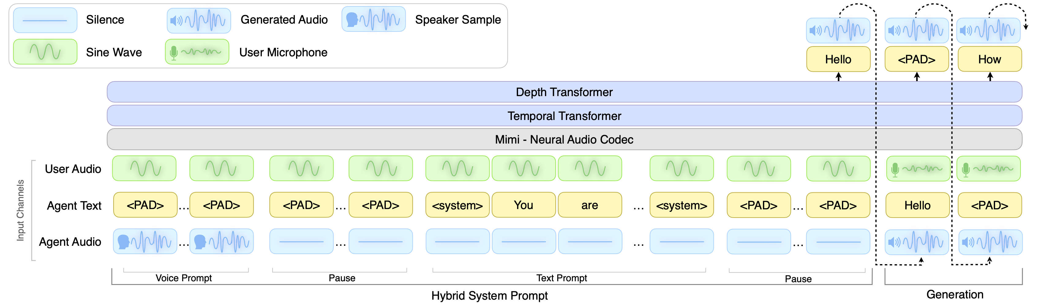
Figure 3: PersonaPlex architecture diagram showing voice and role conditioning built on top of the Moshi full duplex speech to speech foundation model.^[8]

The Emerging Landscape of Speech Foundation Models

The success of Moshi catalyzed rapid progress across the field, with several open source foundation models pushing the boundaries of what speech to speech systems can achieve. Three models in particular illustrate the trajectory from early prototypes to production ready multimodal systems.

SpeechGPT (Zhang et al., 2023)^[9] was among the first to demonstrate that a single large language model could perceive and generate speech without relying on an external TTS pipeline. The key insight was to discretize speech into tokens using a neural codec, then expand the text vocabulary of an existing LLM to include these speech tokens alongside conventional text tokens. SpeechGPT introduced a three stage training strategy: modality adaptation pretraining to familiarize the LLM with speech tokens, cross-modal instruction fine-tuning to align speech and text capabilities, and chain of modality instruction fine-tuning where the model first generates a text response and then converts it to speech tokens. While the chain of modality approach produced intelligible responses, it required generating the full text answer before beginning speech synthesis, making it incompatible with streaming or realtime interaction. Nonetheless, SpeechGPT established the foundational idea that speech generation could be reframed as a token prediction problem within the same framework used for text, an insight that every subsequent model in this space has built upon.

Mini-Omni (Xie and Wu, 2024)^[10] addressed this streaming limitation directly, becoming the first fully end to end open source model capable of realtime speech interaction. Rather than generating text first and speech second, Mini-Omni proposed a text-instructed speech generation method that produces both modalities simultaneously through batch parallel strategies during inference. The authors also released the VoiceAssistant-400K dataset for fine-tuning models optimized for speech output, and introduced the “Any Model Can Talk” training method that enables existing language models to gain realtime speech capabilities with minimal degradation to their original text abilities. This work demonstrated that the latency penalty of chain of modality was not an inherent limitation of speech LLMs but rather a design choice that could be engineered away.

Qwen2.5-Omni (Xu et al., 2025)^[11] represents the current state of the art among open source multimodal models with speech generation capabilities. Developed by the Qwen team at Alibaba, this end to end model perceives text, images, audio, and video while simultaneously generating text and natural speech in a streaming fashion. The architecture introduces two innovations worth examining in detail. The Thinker-Talker design separates reasoning from speech production: the Thinker component, built on a standard Transformer backbone, processes all input modalities and generates text tokens encoding the semantic content of the response, while the Talker component, a dual track autoregressive model, converts those text tokens into discrete speech tokens in real time. This separation means the computationally expensive reasoning happens once in the Thinker, and the Talker can operate with much lower latency to produce streaming audio output. The second innovation is TMRoPE (Time-aligned Multimodal Rotary Position Embeddings), which extends the standard RoPE position encoding to synchronize timestamps across video and audio inputs, maintaining temporal coherence when the model must reason jointly about what it sees and hears. Qwen2.5-Omni achieves state of the art results on the OmniBench multimodal benchmark and demonstrates speech instruction following performance comparable to text only input on benchmarks like MMLU and GSM8K. The model is available in both 7B and 3B parameter variants under the Apache 2.0 license, with quantized versions (GPTQ-Int4, AWQ) that reduce GPU memory consumption by over 50% while maintaining comparable performance.

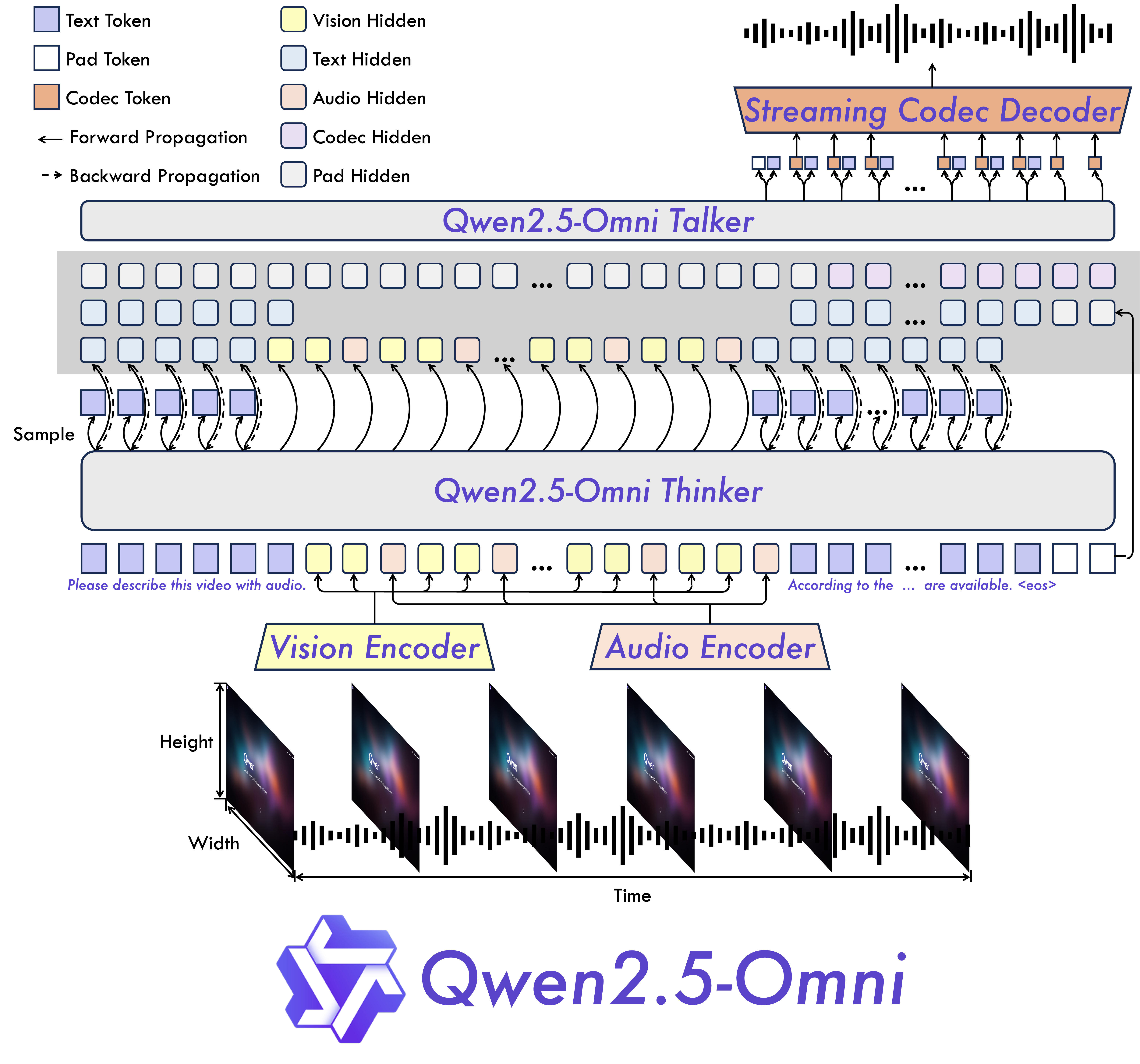
Figure 4: Qwen2.5-Omni architecture showing the Thinker-Talker design with TMRoPE for time aligned multimodal processing. The Thinker handles reasoning across text, image, audio, and video modalities, while the Talker generates streaming speech output through a dual track autoregressive decoder.^[11]

Future Predictions and Directions

The trajectory of S2S foundation models over the next few years points toward increasingly unified architectures. We are already seeing early signals of this convergence in models like VALL-E^[5] and VoiceBox^[6], which treat speech generation as a language modeling problem over discrete audio tokens rather than continuous spectrograms. This codec based paradigm collapses the traditional four stage pipeline into a single autoregressive or masked sequence model, drastically simplifying training and enabling emergent capabilities like in-context learning for voice cloning. As these approaches mature, the distinction between content encoding, speaker conditioning, and waveform synthesis will likely blur into a single end to end system that jointly optimizes all objectives. Diffusion based S2S models represent another promising frontier, offering control over speaking style, emotion, and prosody through classifier free guidance while producing audio quality that rivals or exceeds GAN-based vocoders.

Beyond architecture, several practical challenges will shape the field’s direction in the coming years. realtime streaming has seen remarkable progress with Moshi achieving 200 millisecond practical latency^[7] and Qwen2.5-Omni enabling streaming multimodal interaction on consumer GPUs^[11], but significant challenges remain for truly robust conversational systems that must handle noisy environments, diverse accents, and unstable network connections. Advances in speculative decoding, chunk-wise processing, and efficient attention mechanisms (for a deeper dive into attention optimization, see my earlier post on Key-Value Caching in Large Language Models) will be critical for bridging this gap. Multilingual and code switched S2S presents another frontier, where systems must seamlessly handle mid sentence language switches while preserving speaker identity across languages. Privacy and ethical considerations will also demand attention, as the same voice cloning capabilities that enable creative applications can be misused for impersonation and audio deepfakes. The community will increasingly need robust speaker verification, audio watermarking, and consent frameworks to ensure that these powerful technologies are deployed responsibly.

References

1. Oppenheim, A. V. (1999). Discrete-time signal processing. Pearson Education India.

2. Vaswani, A., Shazeer, N., Parmar, N., et al. (2017). Attention Is All You Need. Advances in Neural Information Processing Systems (NeurIPS).

3. Wan, L., Wang, Q., Papir, A., & Moreno, I. L. (2018). Generalized End-to-End Loss for Speaker Verification. ICASSP.

4. Kong, J., Kim, J., & Bae, J. (2020). HiFi-GAN: Generative Adversarial Networks for Efficient and High Fidelity Speech Synthesis. NeurIPS.

5. Wang, C., Chen, S., Wu, Y., et al. (2023). Neural Codec Language Models are Zero-Shot Text to Speech Synthesizers (VALL-E). arXiv preprint arXiv:2301.02111.

6. Le, M., Vyas, A., Shi, B., et al. (2024). Voicebox: Text-Guided Multilingual Universal Speech Generation at Scale. NeurIPS.

7. Défossez, A., Mazaré, L., Orsini, M., et al. (2024). Moshi: a speech-text foundation model for realtime dialogue. arXiv preprint arXiv:2410.00037.

8. Roy, A., Raiman, J., Lee, J., et al. (2025). PersonaPlex: Voice and Role Control for Full Duplex Conversational Speech Models. arXiv preprint arXiv:2602.06053.

9. Zhang, D., Li, S., Zhang, X., et al. (2023). SpeechGPT: Empowering Large Language Models with Intrinsic Cross-Modal Conversational Abilities. Findings of EMNLP.

10. Xie, Z. & Wu, C. (2024). Mini-Omni: Language Models Can Hear, Talk While Thinking in Streaming. arXiv preprint arXiv:2408.16725.

11. Xu, J., Guo, Z., He, J., et al. (2025). Qwen2.5-Omni Technical Report. arXiv preprint arXiv:2503.20215.

12. Cui, W., Yu, D., Jiao, X., et al. (2024). Recent Advances in Speech Language Models: A Survey. ACL 2025.