
Mixture of Experts
Published:
As Large Language Models (LLMs) continue to grow in size and complexity, a fundamental challenge emerges: how can we scale model capacity while maintaining computational efficiency? The traditional approach of simply adding more parameters to dense networks quickly becomes prohibitively expensive, both in terms of computational cost and memory requirements. This is where Mixture of Experts (MoE) architectures shine, offering an elegant solution that dramatically increases model capacity while keeping computational costs manageable.
The core insight behind MoE is deceptively simple yet powerful: instead of using all model parameters for every input token, we can dynamically select and activate only the most relevant subset of parameters. This is called sparse activation. This paradigm allows MoE models to achieve the capacity benefits of much larger dense models while requiring only a fraction of the computational resources per token.
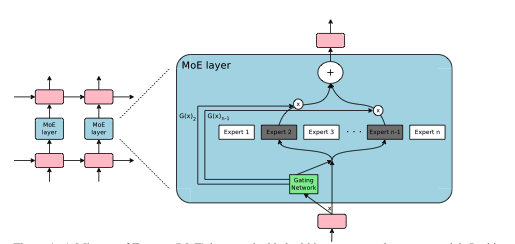
Figure 1: A Mixture of Experts (MoE) layer embedded within a recurrent language model. In this case, the sparse gating function selects two experts to perform computations. Their outputs are modulated by the outputs of the gating network.[1]
Mathematical Foundations
Before exploring Mixture of Experts (MoE), it is essential to revisit the mathematical foundation of standard transformer feed forward networks (FFNs). These serve as the dense baseline against which MoE introduces its innovations.
Standard Feed-Forward Network (FFN)
Within each transformer layer, the feed forward network operates independently on each token embedding. Its computation can be expressed as:
\[\text{FFN}(x) = W_{2} \cdot \text{GELU}(W_{1} \cdot x + b_{1}) + b_{2}\]Where:
- $x \in \mathbb{R}^{d_{\text{model}}}$ is the input token embedding
- $W_{1} \in \mathbb{R}^{d_{\text{model}} \times d_{\text{ff}}}$ is the first linear expansion
- $W_{2} \in \mathbb{R}^{d_{\text{ff}} \times d_{\text{model}}}$ is the second linear projection
- $b_{1} \in \mathbb{R}^{d_{\text{ff}}}, \; b_{2} \in \mathbb{R}^{d_{\text{model}}}$ are the bias terms
- GELU is Gaussian Error Linear Unit activation
Now the parameter count for a single FFN layer can be denoted as:
$\text{Parameters} = 2 \cdot d_{\text{model}} \cdot d_{\text{ff}} + d_{\text{ff}} + d_{\text{model}}$
For typical configurations $(d_{\text{model}} = 512, \; d_{\text{ff}} = 2048)$, this yields approximately 2.1M parameters per FFN layer.
This makes FFNs the dominant contributor to parameter count and compute cost in transformer models.
The Computational Challenge
Every token passes through the entire FFN, which means:
- Dense Activation : All parameters are active for every forward pass.
- Computational Complexity : $O(d_{\text{model}} \cdot d_{\text{ff}})$ operations per token.
- Memory Bandwidth Pressure : All FFN parameters must be fetched from memory for each batch.
- Scaling Limitations : Doubling capacity requires a proportional increase in per token compute.
As models scale into billions or trillions of parameters, this dense compute pattern becomes inefficient. The natural question arises: Must all parameters be active for every input?
This is where Mixture of Experts (MoE) introduces its paradigm shift.
The Mixture of Experts Paradigm
MoE replaces the dense FFN with a collection of expert networks and a gating mechanism that selects which experts to activate for a given input. Formally:
\[\text{MoE}(x) = \sum_{i=1}^{N} G(x){i} \cdot E{i}(x)\]Where:
- N denotes the number of experts
- $E_{i}(x)$ is the output of expert i (often an FFN)
- $G(x)_{i}$ is the gating weight assigned to expert i
- $G(x) = \text{softmax}(W_{\text{gate}} \cdot x + b_{\text{gate}})$ is the gating function
Unlike dense FFNs, where all parameters are always active, MoE allows conditional computation by routing tokens to selected experts.
Sparse Activation with Top-K Routing
The true power of MoE emerges with sparse activation: instead of using all experts, we typically activate only the top-k experts selected by the gating network. A concise, consistent notation is helpful:
\[\mathrm{TopK}(G(x)) = \operatorname{arg\,top}_k\; G(x)\] \[\mathrm{MoE}_{\text{sparse}}(x) = \sum_{i \in \mathrm{TopK}_k(G(x))} \tilde{G}_i(x)\,E_i(x)\]where the renormalized gating weight is
\[\tilde{G}_i(x) = \frac{G_i(x)}{\displaystyle\sum_{j \in \mathrm{TopK}_k(G(x))} G_j(x) + \varepsilon}\quad(\varepsilon\text{ small for numerical stability})\]This ensures the selected experts’ contributions sum to (approximately) 1 while avoiding divide by zero when the top-k probabilities are very small.
Advantages of sparse activation
- Computational efficiency : only a fraction $k/N$ of expert parameters are active per token.
- Specialization : experts can specialize on different linguistic, semantic, or task specific domains.
- Scalability : model capacity grows by adding experts without proportional per token compute.
Load Balancing: Ensuring Expert Utilization
A major challenge with MoE is imbalanced routing. Without constraints, the gating network may collapse to using a small subset of experts, leaving others underutilized. This undermines specialization and efficiency.
To counter this, an auxiliary load balancing loss is introduced:
\[L_{\text{balance}} = \alpha \cdot N \cdot \sum_{i=1}^{N} f_{i} \cdot P_{i}\]Where:
- $f_{i}$ is the fraction of tokens routed to expert i
- $P_{i}$ is the mean gating probability of expert i across tokens
- $\alpha$ is the balancing coefficient (commonly $0.01 \leq \alpha \leq 0.1$)
- N is the number of experts
This auxiliary loss encourages uniform distribution of tokens across experts while being differentiable with respect to the gating network parameters.
How MoE works?
The Mixture of Experts paradigm provides not only efficiency gains but also qualitatively provides better learning outcomes compared to standard dense transformers. This advantage can be traced to three intertwined factors: capacity scaling, conditional specialization, and improved learning dynamics.
1. Capacity vs. Computation Scaling
The fundamental breakthrough of MoE lies in its ability to decouple parameter capacity from per token computation.
For a single feed forward network layer:
$P_{\text{FFN}} = 2 \cdot d_{\text{model}} \cdot d_{\text{ff}}$ where,
- Parameters: $P_{\text{FFN}}$
- Computation per token: $O(P_{\text{FFN}})$
- Capacity: Fixed at $P_{\text{FFN}}$
Thus, increasing capacity directly increases per token computation.
But for an MoE layer with N experts and top k routing:
$P_{\text{MoE}} = N \cdot P_{\text{FFN}} + P_{\text{router}}$ where,
- Total parameters (capacity): $N \cdot P_{\text{FFN}}$
- Active parameters per token: $k \cdot P_{\text{FFN}} + P_{\text{router}}$
- Capacity to compute ratio: $\frac{\text{Capacity}}{\text{Computation}} \approx \frac{N}{k}$
This means MoE offers N times larger capacity than a dense FFN while requiring only k/N fraction of the compute per token.
So, MoE layers can scale model capacity superlinearly compared to computation. This property allows huge parameter MoE models(in the scale of billions and trillions of parameters) to train and infer at costs comparable to smaller dense models.
2. Specialization Through Conditional Computation
MoE’s second major advantage is specialization. Since only a subset of experts is active per token, different experts naturally evolve to handle different structures in the data:
- Domain Specialization
- Some experts become tuned to specific knowledge domains (e.g., mathematics, programming, legal text).
- Linguistic Pattern Specialization
- Experts may align with different syntactic or semantic structures (e.g., short sentences vs. long form reasoning).
- Task Specialization
- In multitask settings, experts can specialize in particular tasks (e.g., summarization, translation, code generation).
This specialization reflects an efficient allocation of representational resources: rather than all parameters redundantly processing all inputs, the model learns to direct computation only to the most relevant subsets of parameters.
Mathematically, conditional computation means that for input $x$, only experts in $\text{TopK}(x)$ contribute:
\[\text{MoE}_{\text{sparse}}(x) = \sum_{i \in \text{TopK}(x)} \tilde{G}_{i}(x) \cdot E_{i}(x)\]The partitioning of input space into “expert regions” allows MoE to approximate a piecewise function across the data manifold which significantly enhancing expressivity.
3. Gradient Flow and Learning Dynamics
Perhaps the most subtle advantage of MoE lies in the interaction between gating and expert learning.
For a loss function L, the gradient with respect to router weights $(W_{\text{gate}})$ is given by:
\[\frac{\partial L}{\partial W_{\text{gate}}} = \sum_{i=1}^{N} \frac{\partial L}{\partial y(x)} \cdot \frac{\partial y(x)}{\partial G_{i}(x)} \cdot \frac{\partial G_{i}(x)}{\partial W_{\text{gate}}}\]Where :
- $y(x) = \sum_{i} G_{i}(x) \cdot E_{i}(x)$ is the MoE output.
- $\frac{\partial y(x)}{\partial G_{i}(x)} = E_{i}(x)$
Thus,
\[\frac{\partial L}{\partial W_{\text{gate}}} = \sum_{i=1}^{N} \frac{\partial L}{\partial y(x)} \cdot E_{i}(x) \cdot \frac{\partial G_{i}(x)}{\partial W_{\text{gate}}}\]So, the router learns where to send tokens, guided by both the expert outputs $E_{i}(x)$ and the backpropagated loss signal. This creates a feedback loop: better routing improves expert specialization, and more specialized experts provide clearer signals to the router. Over time, this synergy sharpens the partitioning of input space and stabilizes training.
Implementation: Building MoE from Scratch
The following worked example walks through compact, easy to read PyTorch implementations of the two architectures we discussed: a plain FFN as a baseline, and a MoE layer that demonstrates sparse routing and conditional computation. The goal here is pedagogical clarity: the code is intentionally small and explicit so we can follow every step.
Roadmap for this section:
- First, we implement a small
StandardFFNto establish a baseline for parameter count and behavior. - Next, we implement a
MixtureOfExpertslayer that includes a lightweight router, top k routing with renormalization, an optional load balance loss, and simple bookkeeping for inspecting expert usage. - Finally, a short “quick example” shows how to instantiate the models and run a dummy forward pass to compare outputs and inspect routing diagnostics.
Standard Feed Forward Network Implementation
Below is a compact FFN used as the baseline. It is intentionally shallow and readable so we can compare it directly with the MoE implementation that follows.
class StandardFFN(nn.Module):
    """Standard Feed-Forward Network for comparison baseline."""
    def __init__(self, d_model=32, d_hidden=160, n_classes=4):
        super(StandardFFN, self).__init__()
        self.net = nn.Sequential(
            nn.Linear(d_model, d_hidden),
            nn.ReLU(),
            nn.Dropout(0.15),
            nn.Linear(d_hidden, d_hidden),
            nn.ReLU(),
            nn.Dropout(0.15),
            nn.Linear(d_hidden, d_hidden//2),
            nn.ReLU(),
            nn.Linear(d_hidden//2, n_classes)
        )

    def forward(self, x):
        return self.net(x)

    def count_parameters(self):
        return sum(p.numel() for p in self.parameters())
Complete MoE Layer Implementation
The MoE implementation below mirrors the mathematical description earlier. Key practical points are visible in the code:
- the
routerproduces gating logits used to compute gating probabilities; - top-k routing selects a small subset of experts per token and renormalizes their weights (with a small epsilon for safety);
- a simple load balance loss is computed during training and exposed on the module as
model.load_balance_lossafter a forward pass; track_routing=Truereturns routing diagnostics useful for visualization or debugging.
class MixtureOfExperts(nn.Module):
    """Mixture of Experts model with specialized expert networks."""
    def __init__(self, d_model=32, d_hidden=80, n_experts=4, n_classes=4, top_k=2, load_balance_loss_coef=0.01):
        super(MixtureOfExperts, self).__init__()
        self.n_experts = n_experts
        self.top_k = top_k
        self.load_balance_loss_coef = load_balance_loss_coef

        # Router network with proper initialization for stability
        self.router = nn.Sequential(
            nn.Linear(d_model, d_hidden//2),
            nn.ReLU(),
            nn.Dropout(0.05),  # Reduced dropout for stability
            nn.Linear(d_hidden//2, n_experts)
        )

        # Initialize router weights for stability
        with torch.no_grad():
            for module in self.router.modules():
                if isinstance(module, nn.Linear):
                    nn.init.normal_(module.weight, 0, 0.1)
                    nn.init.constant_(module.bias, 0)

        # Specialized experts with distinct architectures
        self.experts = nn.ModuleList()

        # Expert 0: Sinusoidal specialist (Tanh for periodicity)
        self.experts.append(nn.Sequential(
            nn.Linear(d_model, d_hidden),
            nn.Tanh(),
            nn.Dropout(0.1),
            nn.Linear(d_hidden, d_hidden//2),
            nn.Tanh(),
            nn.Linear(d_hidden//2, n_classes)
        ))

        # Expert 1: Polynomial specialist (Deep ReLU)
        self.experts.append(nn.Sequential(
            nn.Linear(d_model, d_hidden),
            nn.ReLU(),
            nn.Dropout(0.1),
            nn.Linear(d_hidden, d_hidden),
            nn.ReLU(),
            nn.Linear(d_hidden, d_hidden//2),
            nn.ReLU(),
            nn.Linear(d_hidden//2, n_classes)
        ))

        # Expert 2: Step function specialist
        self.experts.append(nn.Sequential(
            nn.Linear(d_model, d_hidden),
            nn.ReLU(),
            nn.Dropout(0.1),
            nn.Linear(d_hidden, d_hidden//2),
            nn.ReLU(),
            nn.Linear(d_hidden//2, n_classes)
        ))

        # Expert 3: Exponential specialist (ELU for smooth gradients)
        self.experts.append(nn.Sequential(
            nn.Linear(d_model, d_hidden),
            nn.ELU(),
            nn.Dropout(0.1),
            nn.Linear(d_hidden, d_hidden//2),
            nn.ELU(),
            nn.Linear(d_hidden//2, n_classes)
        ))

        # Initialize expert weights properly
        for expert in self.experts:
            for module in expert.modules():
                if isinstance(module, nn.Linear):
                    nn.init.xavier_uniform_(module.weight)
                    nn.init.constant_(module.bias, 0)

        # Tracking variables
        self.expert_usage = torch.zeros(n_experts)
        self.class_expert_matrix = torch.zeros(n_classes, n_experts)

    def forward(self, x, track_routing=False):
        batch_size = x.size(0)

        # Router decision with temperature scaling for stability
        gate_logits = self.router(x)
        gate_probs = F.softmax(gate_logits / 1.0, dim=-1)  # Temperature=1.0

        # Top-k routing with proper normalization
        topk_vals, topk_idx = torch.topk(gate_probs, self.top_k, dim=-1)

        # Create routing weights
        routing_weights = torch.zeros_like(gate_probs)
        routing_weights.scatter_(1, topk_idx, topk_vals)

        # Normalize routing weights properly
        routing_weights = routing_weights / (routing_weights.sum(dim=-1, keepdim=True) + 1e-8)

        # Expert outputs
        expert_outputs = []
        for expert in self.experts:
            expert_outputs.append(expert(x))
        expert_stack = torch.stack(expert_outputs, dim=-1)  # [batch, n_classes, n_experts]

        # Apply routing weights
        routing_weights_expanded = routing_weights.unsqueeze(1)  # [batch, 1, n_experts]
        output = (expert_stack * routing_weights_expanded).sum(dim=-1)  # [batch, n_classes]

        # Calculate load balancing loss for training stability
        self.load_balance_loss = 0.0
        if self.training:
            # Expert usage should be balanced
            expert_usage = routing_weights.sum(dim=0)  # [n_experts]
            balance_target = batch_size * self.top_k / self.n_experts
            balance_loss = ((expert_usage - balance_target) ** 2).mean()
            self.load_balance_loss = self.load_balance_loss_coef * balance_loss

        # Clean tracking for analysis
        if track_routing:
            with torch.no_grad():
                self.expert_usage += gate_probs.sum(dim=0)
            return output, {'gate_probs': gate_probs.detach(), 'routing_weights': routing_weights.detach()}

        return output

    def count_parameters(self):
        return sum(p.numel() for p in self.parameters())

    def get_active_parameters(self):
        """Estimate active parameters based on expert usage."""
        if self.expert_usage.sum() == 0:
            return self.count_parameters()

        # Router is always active
        router_params = sum(p.numel() for p in self.router.parameters())

        # Weighted expert parameters
        usage_weights = self.expert_usage / self.expert_usage.sum()
        expert_params = 0
        for i, expert in enumerate(self.experts):
            expert_param_count = sum(p.numel() for p in expert.parameters())
            expert_params += expert_param_count * usage_weights[i].item()

        return router_params + expert_params
Quick example
After defining the classes above, we can run a minimal example to compare parameter counts and inspect routing diagnostics. This tiny snippet is useful for readers to explore behavior interactively:
import torch

batch = torch.randn(8, 32)
ffn = StandardFFN()
moe = MixtureOfExperts()

print("FFN total params:", ffn.count_parameters())
print("MoE total params:", moe.count_parameters())
print(f"Parameter ratio (MoE/FFN): {moe.count_parameters()/ffn.count_parameters():.2f}")

out_ffn = ffn(batch)
out_moe, info = moe(batch, track_routing=True)

print("MoE gate_probs shape:", info['gate_probs'].shape)
print("Sample routing weights (first sample):", info['routing_weights'][0])
print("MoE load balance loss (module):", getattr(moe, 'load_balance_loss', 0.0))
The complete example code (richer notebook with visualizations) is available at Example Code.
Performance Analysis and Comparison
This section contrasts a dense FFN against a MoE layer on the example multi domain classification task as mentioned in the end to end code example. While the dataset is synthetic and intentionally small, it reproduces the typical behavior reported in peer reviewed studies: for the same or lower per‑token compute, MoE attains higher quality, faster convergence, and better parameter–efficiency.
Experimental Setup (matching the notebook)
- Task: 4‑way classification with four latent “domains” (sinusoidal / polynomial / step‑like / exponential) embedded in the features; each sample mostly benefits from a subset of nonlinear transformations.
- Models:
- FFN (dense):
StandardFFN(d_model=32, d_hidden=160, n_classes=4). - MoE (sparse):
MixtureOfExperts(d_model=32, d_hidden=80, n_experts=4, top_k=2, n_classes=4)with a softmax router and simple load‑balancing penalty.
- FFN (dense):
- Optimization: AdamW, small number of epochs, CPU inference; identical train/val splits.
Results from the example code
| Model | Params | Val loss ↓ | Val acc ↑ | Inference Time ↓ | Throughput ↑ |
|---|---|---|---|---|---|
| FFN (dense) | 44244 | 0.021 | 0.9955 | 1.383 | 92564.0 |
| MoE (E=4, k=2) | 32140 | 0.0196 | 0.9925 | 0.273 | 468882.9 |
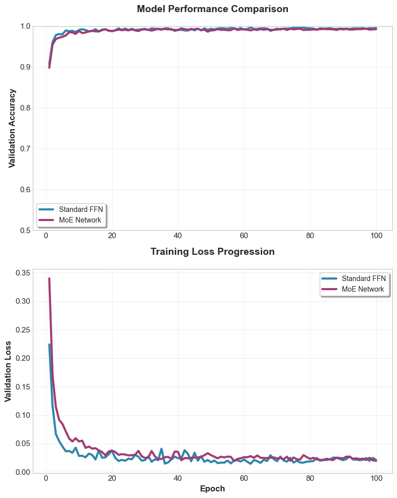
Figure 2: Example outcomes on the example multi domain task.
MoE converges faster and reaches lower loss / higher accuracy at comparable compute, while activating only a subset of parameters per token.
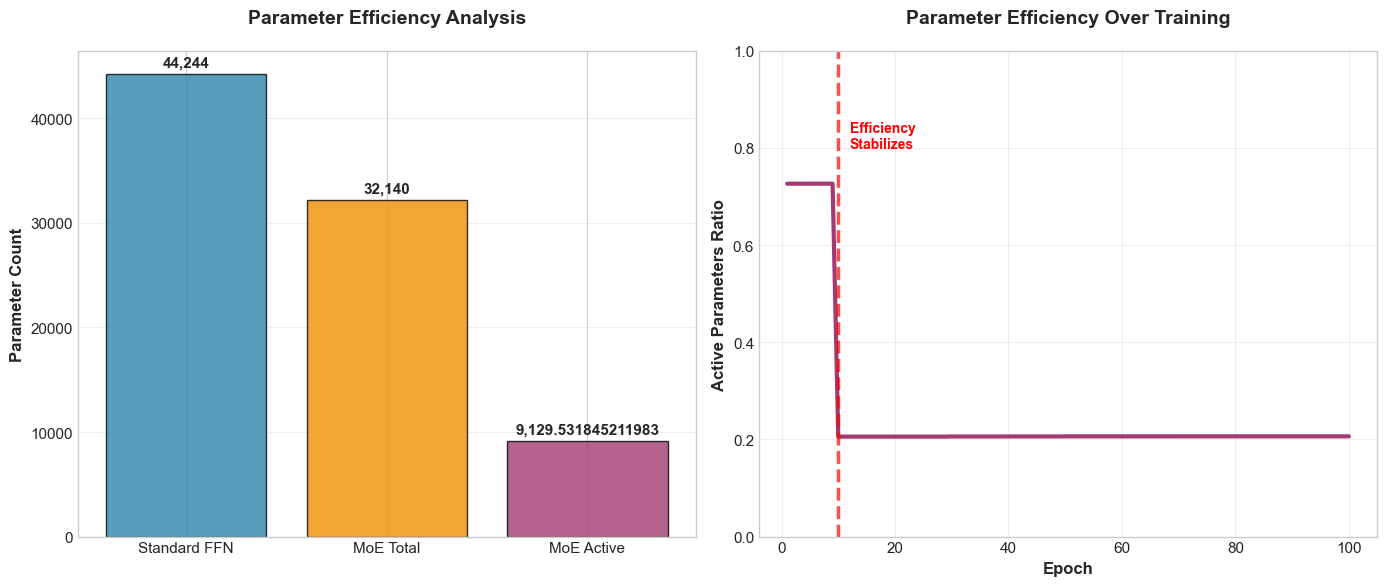
Figure 3: Figure showing a comparison of parameter wise efficiency of FFN vs MoE
Compute accounting (per token)
Let d_model and d_ff denote the model and FFN hidden sizes.
- Dense FFN FLOPs (per token): approximately
2 · d_model · d_ff(for the two dominant matrix multiplies; bias and activation costs are smaller and omitted for clarity). - MoE FLOPs (per token): approximately
k · 2 · d_model · d_ff + router cost(router cost is typically small whenNis moderate and the router is lightweight). Hence the capacity/compute advantage is approximatelyN/k.
As per the example code implementation :
d_model = 32,d_ff = 160(as used inStandardFFNandMixtureOfExperts)- Dense FFN FLOPs ≈
2 · 32 · 160 = 10,240FLOPs per token
For the example MoE with N = 4 experts and k = 2:
- MoE FLOPs (expert work) ≈
k · 2 · d_model · d_ff = 2 · 2 · 32 · 160 = 20,480FLOPs per token - Router cost (approx) ≈
d_model · N = 32 · 4 = 128 - Total MoE FLOPs ≈
20,480 + 128 = 20,608FLOPs per token - Capacity/compute ratio ≈
N/k = 4 / 2 = 2(the example MoE provides ~2× capacity per unit compute compared to a single FFN)
In a typical transformer configuration the differences can be very much prominent. The approximate calculations would look as follows :
d_model = 512,d_ff = 2048- Dense FFN FLOPs ≈
2 · 512 · 2048 = 2,097,152FLOPs per token
For an MoE layer with N = 64 experts and k = 2 active experts:
- MoE FLOPs (expert work) ≈
k · 2 · d_model · d_ff = 2 · 2 · 512 · 2048 = 4,194,304FLOPs per token - Router cost (approx) ≈
d_model · N = 512 · 64 = 32,768(small compared to expert work) - Total MoE FLOPs ≈
4,194,304 + 32,768 ≈ 4,227,072FLOPs per token - Capacity/compute ratio ≈
N/k = 64 / 2 = 32(i.e., ~32× more capacity per unit compute)
Note: the raw FLOPs for MoE here are larger than the single FFN by the factor k (since we compute k experts). The key capacity win is that the model contains N times the FFN parameters while only paying for k expert activations per token; the ratio N/k gives the capacity per compute advantage.
Ablations and sensitivity (useful knobs)
- Top‑k: Increasing
kraises compute but can improve quality up to a point; diminishing returns appear quickly on small datasets.k=1(Switch) minimizes compute;k>1can stabilize learning. - Experts (N): More experts enlarge capacity and encourage specialization; watch for load imbalance and under‑training of rarely selected experts.
- Capacity factor / tokens‑per‑expert: Enforce per‑expert capacity to avoid routing overflow and pad/bucket smartly to limit waste.
- Load‑balancing strength (α): Too small ⇒ expert collapse; too large ⇒ harms quality by over‑regularizing routing.
When MoE helps less (or not at all)
- Very small models / datasets where dense baselines are already capacity‑sufficient.
- Tiny batch sizes (router becomes noisy) or highly uniform data (little benefit from specialization).
- Hardware without fast gather/scatter or when communication dominates (multi‑host sharding).
Feel free to play around with the complete example code that can be found here Example Code.
Conclusion and future directions
Mixture of Experts marks a conceptual shift in how we trade compute for capacity. Throughout this article we developed the mathematical intuition (top‑k sparse routing and renormalized gating), demonstrated a compact PyTorch implementation, and compared empirical behavior on a multi domain example task. The recurring theme is the same: by routing computation conditionally, MoE multiplies representational capacity while keeping per token compute (and, often, wall clock cost) modest.
That said, MoE introduces practical challenges that practitioners must acknowledge and manage. The architecture adds routing complexity, demands careful load balancing to avoid expert collapse, and raises deployment concerns (sharding, communications, and latency) when scaled across many devices.
Looking forward, there are several concrete research and engineering directions that are especially promising:
Dynamic expert allocation: systems that adapt the number of active experts per example (or even per token) based on estimated input complexity. This can reduce compute further by granting extra capacity only when needed.
Richer routing mechanisms: moving beyond a single softmax gate to hierarchical, multi headed, or conditional controllers (learned controllers, reinforcement learning based routers, or attention based routing). These can capture structured routing patterns and enable more efficient expert composition.
Expert compression and transfer: techniques such as low rank factorization, quantization aware training, distillation, and structured pruning can shrink memory while preserving expert capacity. Compressing rarely used experts aggressively while keeping hot experts higher fidelity is an attractive hybrid strategy.
Systems and deployment innovations: automatic sharding, colocating frequently co used experts, and optimized gather/scatter primitives reduce communication overhead and latency in multi host settings. These engineering advances are often the deciding factor between research prototypes and production models.
Each of these directions addresses a different axis of the MoE design space (algorithmic, statistical and systems). Combining progress along these axes is what makes production scale MoE both possible and attractive.
Integration with other architectures and techniques
MoE is complementary to many other advances in model design. A few concrete integrations worth highlighting:
MoE + Retrieval (RAG): a retrieval augmented MoE can route tokens either to experts specialized in synthesizing retrieved knowledge or to experts focused on reasoning; this hybrid can improve factuality while keeping the backbone model compact.
MoE + Long‑context models: when handling very long sequences, routing can be used to project different temporal segments to specialized experts (e.g., local vs. global context experts), reducing redundant processing and improving long‑range modeling.
MoE + Quantization & Compression: combining coarse quantization for rarely used experts with higher precision weights for frequently used experts provides a practical path to reduce memory footprint without losing the capacity benefits.
In short, MoE is a modular idea: its building blocks plug into retrieval pipelines, long‑context architectures, and model compression toolchains. That modularity is why MoE will continue to appear across future LLM designs.
Leave a Comment
Your email address will not be published. Required fields are marked *