KL Divergence

Understanding Kullback-Leibler divergence

In today’s rapidly evolving artificial intelligence landscape, one mathematical concept stands as a cornerstone across countless applications: the Kullback-Leibler (KL) divergence. With the rise of large language models (Thanks to ChatGPT!), we’ve been fastforwarded into the future, thanks to the countess innovations that has gone in the past. From training large language models to detecting anomalies in real-time data streams, KL divergence has become the silent engine powering some of the most sophisticated AI systems. As we witness unprecedented advances in machine learning, understanding this fundamental measure of distributional difference has never been more crucial for data scientists and ML researchers.

KL divergence, also known as relative entropy, measures how one probability distribution diverges from a reference distribution. What makes this concept particularly fascinating is its asymmetric nature and its deep connections to information theory, making it an ideal tool for comparing learned distributions against target distributions in machine learning contexts.

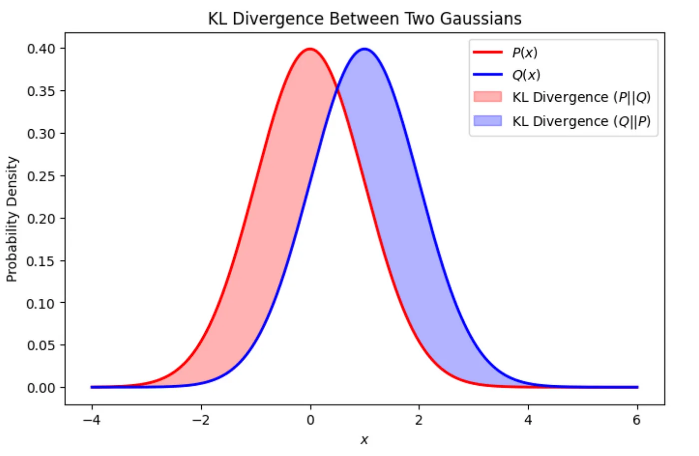
Two Gaussian distributions P(x) and Q(x); the shaded regions indicate the asymmetry of the KL divergence. Forward KL (red area) penalizes when Q assigns zero or low probability to a region where P has high probability and reverse KL (blue area) vice versa.^[7]

Current Applications: Where KL Divergence Powers Modern AI

Reinforcement Learning and Human Feedback (RLHF)

In the realm of large language models, KL divergence serves as a crucial regularization mechanism in RLHF pipelines. When fine-tuning models like Meta’s LLama, researchers employ KL divergence to ensure the updated model doesn’t drift too far from the original pre-trained version. This prevents reward hacking while maintaining the model’s fluency and general capabilities.

The RLHF objective typically includes a KL regularization term:

where $ \pi_{\theta} $ represents the policy being optimized, $ \pi_{ref} $ is the reference model, and $ \beta $ controls the strength of the KL penalty.

Variational Autoencoders and Generative Modeling

In variational autoencoders (VAEs), KL divergence plays a dual role as both a regularizer and a learning objective. The ELBO (Evidence Lower Bound) objective directly incorporates KL divergence:

This formulation ensures that the learned latent representations follow a structured prior distribution while maintaining reconstruction quality.

Model Evaluation and Knowledge Distillation

KL divergence has become the standard metric for knowledge distillation, where smaller student models learn to mimic larger teacher models. The process minimizes:

where $ \tau $ is the temperature parameter that softens the probability distributions.

Mathematical Foundation

Discrete Case

For discrete probability distributions P and Q over a finite set $ \mathcal{X} $, KL divergence is defined as:

Continuous Case

For continuous distributions with probability density functions p(x) and q(x):

Key Properties of KL Divergence

1. Non-negativity: $ D_{KL}(P \parallel Q) \geq 0 $, with equality if and only if P = Q

2. Asymmetry: $ D_{KL}(P \parallel Q) \neq D_{KL}(Q \parallel P) $ in general

Relationship to Cross-Entropy

Before diving into the relationship, let’s briefly recall what cross-entropy is.

What is Cross-Entropy?

Cross-entropy is a widely used loss function in classification problems. It measures the dissimilarity between two probability distributions—typically, the true distribution P (often represented as one-hot labels) and the predicted distribution Q (the output from a model, such as a softmax layer).

Formally, the cross-entropy between distributions P and Q is defined as:

This quantifies the average number of bits needed to encode data drawn from P using a code optimized for Q. The better Q approximates P, the lower the cross-entropy.

And what is Entropy?

Entropy is a special case of cross-entropy where the two distributions are the same. It represents the inherent uncertainty in a distribution:

This measures the average amount of “surprise” or information inherent in the true distribution P.

KL divergence connects intimately with cross-entropy:

Here,

• $D_{KL}(P \parallel Q) $ measures the extra cost of encoding samples from P using a code optimized for Q, instead of the true distribution P.
• $H(P, Q)$ is the cross-entropy.
• $H(P)$ is the entropy of P.

This equation shows that KL divergence is the difference between the cross-entropy and the entropy of the true distribution.

But Why This Matters in Machine Learning?

In most classification tasks, we minimize the cross-entropy loss between the true labels and the predicted probabilities. But since the true distribution P (e.g., one-hot encoded labels) is fixed and does not depend on model parameters, minimizing cross-entropy: $\min_Q H(P, Q) $ is equivalent to minimizing the KL divergence: $\min_Q D_{KL}(P \parallel Q) $ because $H(P)$ is constant with respect to $Q$.

This insight explains why cross-entropy is often used as a proxy to KL divergence in machine learning: it’s simpler to compute, yet still drives the model’s predictions Q to approximate the true labels P as closely as possible.

Practical Example: Computing KL Divergence

Let’s walk through a concrete example to illustrate how KL divergence is calculated between two discrete probability distributions.

Given Distributions

We define two distributions over the same set of three events:

• True distribution P: P = [0.1, 0.4, 0.5]
• Approximate distribution Q (e.g., a model prediction): Q = [0.8, 0.15, 0.05]

KL Divergence Formula

For discrete distributions:

Let’s use the above distribution to calculate :

This tells us that, on average, using Q instead of P incurs an additional 1.927 bits of “cost” per symbol.

Let’s see how this looks in code

import numpy as np
from scipy.special import rel_entr

P = np.array([0.1, 0.4, 0.5])
Q = np.array([0.8, 0.15, 0.05])

kl_divergence = np.sum(rel_entr(P, Q)) / np.log(2)

print(f"D_KL(P || Q) = {kl_divergence:.3f} bits")

And the output will be

D_KL(P || Q) = 1.927 bits

KL Divergence is Asymmetric

Now let’s compute $D_{KL}(Q \parallel P)$ by swapping the arguments. The formula would look the following :

I’ll show how the python code would look like :

kl_reverse = np.sum(rel_entr(Q, P)) / np.log(2)
print(f"D_KL(Q || P) = {kl_reverse:.3f} bits")

And with this, we get the following output :

D_KL(Q || P) = 2.022 bits

As we can see, $D_{KL}(P \parallel Q) \neq D_{KL}(Q \parallel P)$. This asymmetry is a fundamental characteristic of KL divergence.

Implementation Considerations for Modern Practitioners

Numerical Stability

When computing KL divergence, especially in deep learning models, numerical stability is critical. Probabilities close to zero can cause instability due to:

• Division by zero
• Taking the logarithm of zero
• Exploding or vanishing gradients

To prevent this, it’s common to use epsilon smoothing and log-space computations. A simple and efficient implementation using numpy is mentioned below :

def stable_kl_divergence(p, q, epsilon=1e-8):
    p_safe = np.clip(p, epsilon, 1.0)
    q_safe = np.clip(q, epsilon, 1.0)
    return np.sum(p_safe * np.log(p_safe / q_safe))

This avoids undefined operations by:

• Clipping values in p and q to a small lower bound (epsilon)
• Ensuring all logarithms and divisions remain well-defined

But why log-space?

If we’re working with log probabilities (as in many deep learning libraries), we can directly compute KL divergence in log-space to reduce floating-point error:

This is particularly useful when computing with softmax outputs or logits in frameworks like TensorFlow and PyTorch. Here, I have mentioned sample implementation using both these frameworks.

Using TensorFlow :

TensorFlow’s tf.keras.losses.KLDivergence expects normal probability distributions, but since we’re working in log-space, we can do the following:

import tensorflow as tf

def kl_divergence_log_space_tf(log_p, log_q):
    """Compute D_KL(P || Q) in log-space"""
    p = tf.exp(log_p)  # Convert log P back to probability space
    kl = tf.reduce_sum(p * (log_p - log_q), axis=-1)
    return kl

Using PyTorch :

PyTorch provides F.kl_div, which operates in log-space and is numerically stable by default. The code would look like the following :

import torch
import torch.nn.functional as F

def kl_divergence_log_space_torch(log_q, p):
    """Compute D_KL(P || Q) where log_q = log(Q), and p is in prob space."""
    kl = F.kl_div(log_q, p, reduction='batchmean', log_target=False)
    return kl

Gradient Computation

When optimizing models via backpropagation, it’s crucial to understand the gradient of KL divergence with respect to model predictions.

For:

• P: true distribution (usually fixed and one-hot encoded)
• Q: model prediction (e.g., softmax output)

The gradient of the KL divergence with respect to $Q_\theta$ is:

However, in the cross-entropy loss context, where P is fixed and Q is parameterized by the model, a simplified and intuitive expression is often used:

And that evaluates to:

So the gradient with respect to the logits is: \(\nabla_{\theta} D_{KL}(P \parallel Q_{\theta}) = Q_{\theta} - P\)

This represents the direction in which to adjust Q to bring it closer to P, and is the same gradient we’d get from minimizing cross-entropy loss.

Most Deep learning frameworks automatically compute gradients using autograd. Still, it’s helpful to know that when using nn.KLDivLoss(reduction='batchmean')

We should pass log probabilities for Q and regular probabilities for P, because it implements the expectation in log-space:

Future Horizons

I have listed some of my predictions below:

Advanced Optimization and Variance Reduction

The future of KL divergence in machine learning will likely see sophisticated variance reduction techniques becoming mainstream. Recent research has introduced Rao-Blackwellized estimators that provably reduce variance while maintaining unbiasedness. These improvements will be crucial as models scale and training becomes more computationally demanding.

Multimodal World Models

As AI systems become increasingly multimodal, KL divergence will play an expanded role in aligning representations across different modalities. Future vision language models will likely employ KL regularization to ensure consistent semantic representations between visual and textual encodings, leading to more robust and interpretable AI systems.

Real-Time Adaptive Systems

The future will mostly see KL divergence powering truly adaptive or self-sustaining AI systems that continuously monitor and adjust to distributional shifts. These systems will employ sliding window approaches with KL divergence to detect concept drift in real time, automatically triggering model updates or interventions.

Conclusion

As artificial intelligence continues its rapid evolution, KL divergence remains a fundamental tool bridging information theory, statistics, and practical machine learning applications. Its unique properties such as asymmetry, information-theoretic interpretation, and computational efficiency make it indispensable for modern AI systems.

For practitioners and researchers, mastering KL divergence isn’t just about understanding a mathematical formula, rather it’s about grasping a fundamental principle that underlies much of modern machine learning. As we venture into an era of increasingly sophisticated AI systems, this understanding will prove invaluable for developing, optimizing, and interpreting the AI technologies that will shape our future.

References

1. Belov, D. I., & Armstrong, R. D. (2011). Distributions of the Kullback-Leibler divergence with applications. British Journal of Mathematical and Statistical Psychology, 64(2), 291-309.

2. Amini, A. et.al. (2024). Better estimation of the KL divergence between language models. arXiv preprint arXiv:2504.10637.

3. Cui, J. et.al. (2025). Generalized Kullback-Leibler divergence loss for deep learning applications. arXiv preprint arXiv:2503.08038.

4. Shannon, C. E. (1948). A mathematical theory of communication. Bell System Technical Journal, 27(3), 379-423.

5. Kullback, S., & Leibler, R. A. (1951). On information and sufficiency. Annals of Mathematical Statistics, 22(1), 79-86.

6. Asperti, A., & Evangelista, D. (2020). Balancing reconstruction error and Kullback-Leibler divergence in variational autoencoders. IEEE Access, 8, 199875-199884.

7. Chen, Y. (2025). Introduction to Kullback-Leibler Divergence. https://medium.com/@yian.chen261/introduction-to-kullback-leibler-divergence-2d76979d1d8c