
Key-Value caching
Published:
What is Key-Value caching?
Key-value caching, as an optimization technique, focuses on improving the efficiency of the inference process in Large Language Models(LLMs) by reusing previously computed states. In simple terms, it’s a way for the model to “remember” previous calculations to avoid re-computing them for every new word it generates.
Imagine you’re having a conversation. You don’t re-process the entire conversation from the beginning every time someone says something new. Instead, you maintain the context and build upon it. KV caching works on a similar principle for LLMs.
To understand this better, we will briefly touch upon the Transformer architecture proposed in the gamous 2017 paper “Attention is All you need”, the foundation of most modern LLMs.
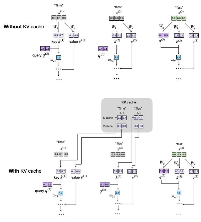
Figure 1: Comparison of text generation with and without KV caching. In the upper panel (no cache), key and value vectors are recalculated at every step, leading to redundant computations. In contrast, the lower panel (with cache) reuses previously stored key and value vectors from the cache, eliminating recomputation and enabling faster inference.[Source : Understanding and Coding the KV Cache in LLMs from Scratch by Sebastian Raschka]
Transformer architecture overview
From a high-level perspective, most transformers consist of a few basic building blocks:
- A tokenizer that splits the input text into subparts, such as words or sub-words.
- An embedding layer that transforms the resulting tokens (and their relative positions within the texts) into vectors.
- A couple of basic neural network layers, including dropout, layer normalization, and regular feed-forward linear layers.
The most innovative of these building blocks is the self-attention mechanism. This mechanism allows the model to weigh the importance of different words in the input sequence when producing the next word. This is where the concepts of Keys and Values originate, and it’s the core of what KV Caching optimizes.
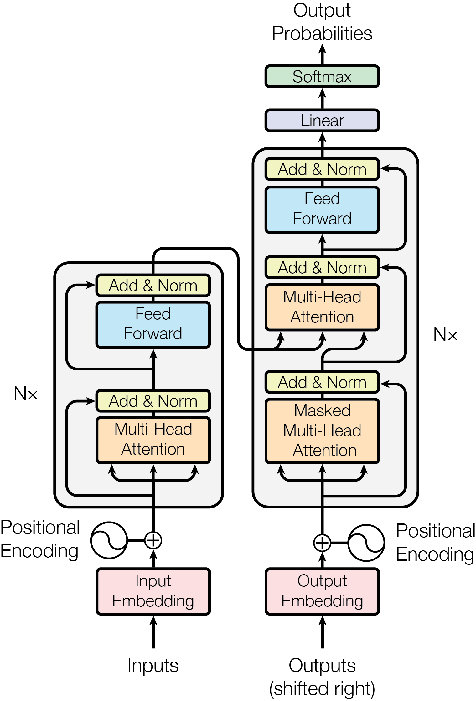
Figure 2: Model Architecture of Transformer[1]
A Closer Look at Self-Attention
Let’s zoom in and understand how self-attention works. For every input token that has been converted into an embedding vector, the model generates three new, distinct vectors:
- Query $(Q)$: Think of this as the current token’s “search query.” It’s looking for relevant information from other tokens in the sequence to better understand its own context.
- Key $(K)$: This is like a “label” or an “index” for a token. It’s what the Query vector from other tokens will match against to find relevant information.
- Value $(V)$: This vector contains the actual substance or meaning of the token. Once a Query finds a relevant Key, the associated Value is what provides the useful information.
These $Q$, $K$, and $V$ vectors are created by multiplying the token’s embedding vector (say $x$) by three separate weight matrices($W^Q, W^K, W^V$). These matrices are learned during the model’s training and are essential for its performance. Basically for an input vector $x$ the process would be :
- $Query = x.W^Q$
- $Key = x.W^K$
- $Value = x.W^V$
The model then uses the Query vector of the current token to score itself against the Key vectors of all tokens in the sequence (including itself). These scores determine how much “attention” to pay to each token’s Value, and this is what makes the model context-aware.
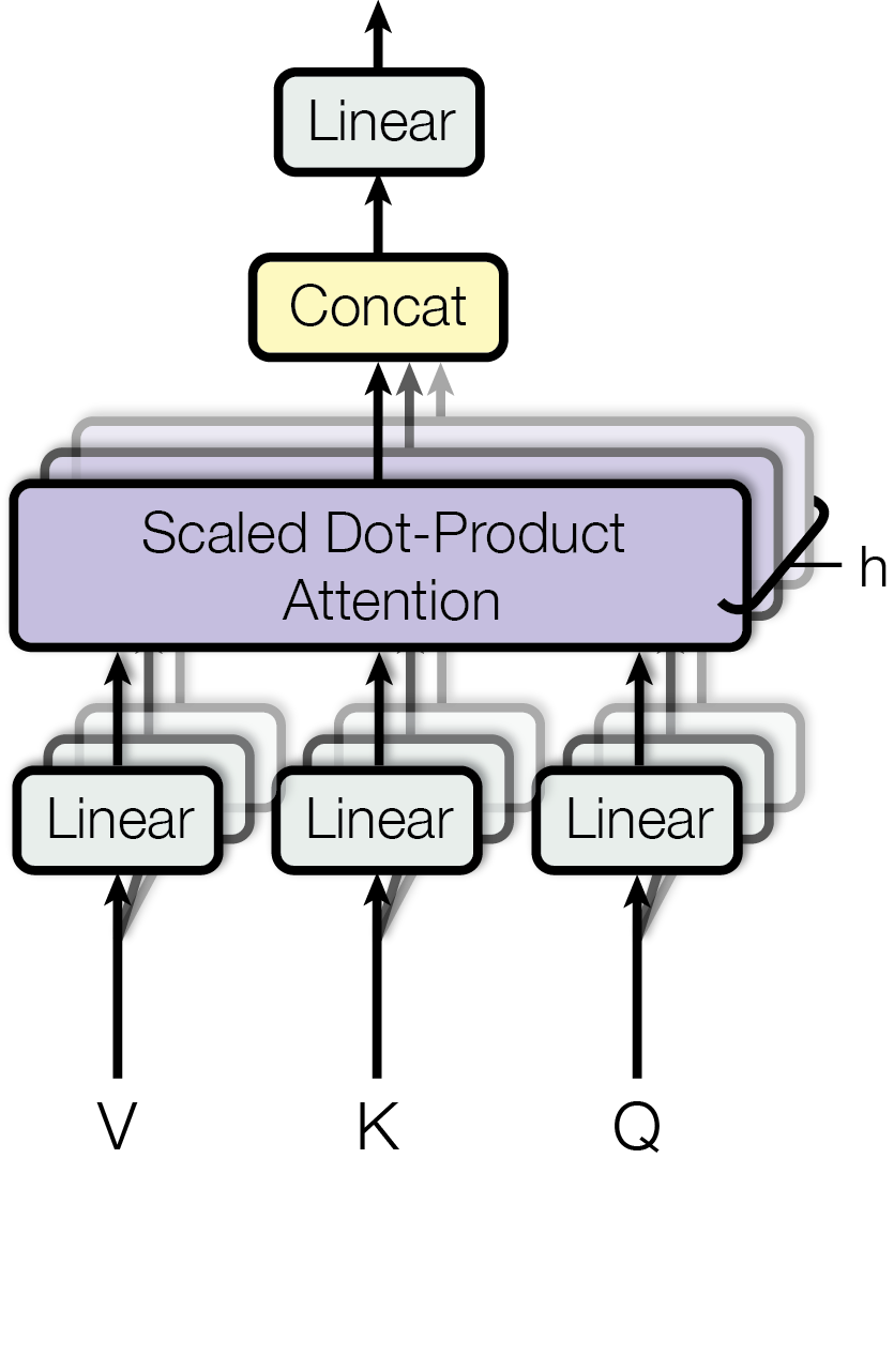
Figure 3: The Multi-Head Attention block in a Transformer[1]
For an input sequence of length $n$ with hidden size $d$, we project the embeddings $X \in \mathbb{R}^{n \times d}$ into Queries, Keys and Values :
\[Q = X W^{Q}, \qquad K = X W^{K}, \qquad V = X W^{V}, \qquad W^{Q}, W^{K}, W^{V} \in \mathbb{R}^{d \times d_h},\]where $d_h = d / h$ is the dimensionality of each of the $h$ attention heads.
Scaled‑dot‑product attention for a single head is then
\[\operatorname{Attention}(Q, K, V) = \operatorname{softmax}\!\left( \frac{Q K^{\mathsf T}}{\sqrt{d_h}} \right) V.\]The matrix product $Q K^{\mathsf T}$ yields an $n \times n$ score matrix whose $(i,j)$-th entry reflects how much token $i$ attends to token $j$.
How Does Key-Value Caching Work?
LLMs generate text in an autoregressive manner, meaning they generate one word at a time, and each new word depends on the previously generated words. Without KV caching, every time the model generates a new word, it would have to recalculate the Key and Value vectors for all the preceding words in the sequence. This is incredibly inefficient and computationally expensive, especially for long sequences of text.
This is where KV caching comes to the rescue.
Instead of discarding the Key and Value vectors after they are calculated, the model stores them in a cache. When generating the next word, the model only needs to calculate the $Q, K$ and $V$ vectors for the newest word and can then retrieve the $K$ and $V$ vectors of all the previous words directly from the cache.
Without KV Caching:
At generation step $t$, the model recomputes keys and values for the entire prefix $x_{1:t}$:
\[\begin{aligned} K^{(t)} &= [\,x_1,\,x_2,\dots, x_t\,] W^{K} \in \mathbb{R}^{t \times d_k},\\[4pt] V^{(t)} &= [\,x_1,\,x_2,\dots, x_t\,] W^{V} \in \mathbb{R}^{t \times d_v}. \end{aligned}\]With the current query $q_t = x_t W^{Q}$, attention is computed as
\[a_t = \operatorname{softmax}\!\left( \frac{q_t {K^{(t)}}^{\!\mathsf T}}{\sqrt{d_h}} \right) V^{(t)}.\]This costs $O(t d_h)$ for projections and another $O(t d_h)$ for the attention matrix–vector product.
With KV Caching:
Key–value caching stores the keys and values from previous steps:
\[K_{\text{cache}}^{(t-1)} \in \mathbb{R}^{(t-1) \times d_k},\qquad V_{\text{cache}}^{(t-1)} \in \mathbb{R}^{(t-1) \times d_v}.\]For the new token $x_t$ we compute only
\[k_t = x_t W^{K}, \qquad v_t = x_t W^{V},\]and append them:
\[\begin{aligned} K_{\text{cache}}^{(t)} &= \operatorname{concat}\bigl( K_{\text{cache}}^{(t-1)},\, k_t \bigr),\\[4pt] V_{\text{cache}}^{(t)} &= \operatorname{concat}\bigl( V_{\text{cache}}^{(t-1)},\, v_t \bigr). \end{aligned}\]Attention for step $t$ becomes
\[a_t = \operatorname{softmax}\!\left( \frac{q_t {K_{\text{cache}}^{(t)}}^{\!\mathsf T}}{\sqrt{d_h}} \right) V_{\text{cache}}^{(t)}.\]The projection cost now drops to $O(d_h)$ (just one token) while the attention term remains $O(t d_h)$, for long prefixes this yields significant speed‑ups in wall‑clock latency.
Let’s walk through an example :
Suppose we want the model to complete the sentence: “The quick brown fox…”
- First Word (“The”): The model processes “The” and calculates its K and V vectors. These are then stored in the KV cache.
- Second Word (“quick”): The model processes “quick.” It calculates the Q vector for “quick” and retrieves the K and V vectors for “The” from the cache. It then calculates the K and V for “quick” and adds them to the cache.
- Third Word (“brown”): The model processes “brown.” It calculates the Q vector for “brown” and retrieves the K and V vectors for “The” and “quick” from the cache. The new K and V for “brown” are also cached.
- Fourth Word (“fox”): The process repeats. The model only needs to compute the Q, K, and V for “fox” and can reuse the cached K and V vectors for “The quick brown.”
This caching mechanism dramatically speeds up the generation of subsequent tokens.
Let’s see it in action
Let us start with implementing a KVCache
import numpy as np
import time
from typing import Tuple, Dict

class KVCache:
    """
    Key-Value cache for transformer attention mechanism with comprehensive tracking
    """
    def __init__(self, max_batch_size: int, max_seq_len: int,
                 n_heads: int, head_dim: int, dtype=np.float16):
        self.max_batch_size = max_batch_size
        self.max_seq_len = max_seq_len
        self.n_heads = n_heads
        self.head_dim = head_dim
        self.dtype = dtype

        # Initialize cache tensors
        cache_shape = (max_batch_size, max_seq_len, n_heads, head_dim)
        self.cache_k = np.zeros(cache_shape, dtype=dtype)
        self.cache_v = np.zeros(cache_shape, dtype=dtype)
        self.cache_len = 0

        # Performance tracking
        self.operations_count = 0
        self.memory_accesses = 0

    def update(self, keys: np.ndarray, values: np.ndarray,
               start_pos: int) -> Tuple[np.ndarray, np.ndarray]:
        """
        Update cache with new key-value pairs

        Args:
            keys: New key tensors [batch_size, seq_len, n_heads, head_dim]
            values: New value tensors [batch_size, seq_len, n_heads, head_dim]
            start_pos: Starting position in the cache

        Returns:
            Updated keys and values including cached ones
        """
        batch_size, seq_len = keys.shape[:2]

        # Store new keys and values in cache
        self.cache_k[:batch_size, start_pos:start_pos + seq_len] = keys
        self.cache_v[:batch_size, start_pos:start_pos + seq_len] = values

        # Update performance counters
        self.operations_count += batch_size * seq_len * self.n_heads * self.head_dim
        self.memory_accesses += 2 * batch_size * seq_len * self.n_heads * self.head_dim

        # Return all keys and values up to current position
        keys_all = self.cache_k[:batch_size, :start_pos + seq_len]
        values_all = self.cache_v[:batch_size, :start_pos + seq_len]

        self.cache_len = start_pos + seq_len
        return keys_all, values_all

    def get_stats(self) -> dict:
        """Get comprehensive cache statistics"""
        element_size = 2 if self.dtype == np.float16 else 4  # bytes per element
        memory_usage = (self.cache_k.size + self.cache_v.size) * element_size
        return {
            'cache_length': self.cache_len,
            'memory_usage_bytes': memory_usage,
            'memory_usage_mb': memory_usage / (1024 * 1024),
            'utilization': self.cache_len / self.max_seq_len,
            'total_operations': self.operations_count,
            'memory_accesses': self.memory_accesses,
            'cache_shape': self.cache_k.shape
        }
Now, let us invoke the KVCache in MultiHead Attention
class MultiHeadAttentionWithCache:
    """
    Multi-head attention with KV caching capability
    """
    def __init__(self, d_model: int, n_heads: int, max_seq_len: int = 2048):
        self.d_model = d_model
        self.n_heads = n_heads
        self.head_dim = d_model // n_heads
        self.scale = 1.0 / (self.head_dim ** 0.5)

        # Initialize weight matrices (normally these would be learned parameters)
        self.w_q = np.random.randn(d_model, d_model) * 0.1
        self.w_k = np.random.randn(d_model, d_model) * 0.1
        self.w_v = np.random.randn(d_model, d_model) * 0.1
        self.w_o = np.random.randn(d_model, d_model) * 0.1

        # Initialize KV cache
        self.kv_cache = None
        self.max_seq_len = max_seq_len

        # Performance tracking
        self.forward_calls = 0
        self.compute_time = 0

    def init_cache(self, batch_size: int):
        """Initialize KV cache for inference"""
        self.kv_cache = KVCache(
            max_batch_size=batch_size,
            max_seq_len=self.max_seq_len,
            n_heads=self.n_heads,
            head_dim=self.head_dim
        )

    def forward(self, x: np.ndarray, start_pos: int = 0,
                use_cache: bool = False) -> np.ndarray:
        """
        Forward pass with optional KV caching

        Args:
            x: Input tensor [batch_size, seq_len, d_model]
            start_pos: Starting position for cache update
            use_cache: Whether to use KV caching
        """
        start_time = time.time()
        self.forward_calls += 1

        batch_size, seq_len, _ = x.shape

        # Compute Q, K, V projections
        q = np.dot(x, self.w_q).reshape(batch_size, seq_len, self.n_heads, self.head_dim)
        k = np.dot(x, self.w_k).reshape(batch_size, seq_len, self.n_heads, self.head_dim)
        v = np.dot(x, self.w_v).reshape(batch_size, seq_len, self.n_heads, self.head_dim)

        if use_cache and self.kv_cache is not None:
            # Update cache and get all keys/values
            k_all, v_all = self.kv_cache.update(k, v, start_pos)
        else:
            k_all, v_all = k, v

        # Transpose for attention computation
        q = np.transpose(q, (0, 2, 1, 3))  # [batch_size, n_heads, seq_len, head_dim]
        k_all = np.transpose(k_all, (0, 2, 1, 3))
        v_all = np.transpose(v_all, (0, 2, 1, 3))

        # Compute attention scores
        scores = np.matmul(q, np.transpose(k_all, (0, 1, 3, 2))) * self.scale

        # Apply softmax
        exp_scores = np.exp(scores - np.max(scores, axis=-1, keepdims=True))
        attn_weights = exp_scores / np.sum(exp_scores, axis=-1, keepdims=True)

        # Apply attention to values
        attn_output = np.matmul(attn_weights, v_all)

        # Reshape and apply output projection
        attn_output = np.transpose(attn_output, (0, 2, 1, 3)).reshape(
            batch_size, seq_len, self.d_model
        )

        output = np.dot(attn_output, self.w_o)

        self.compute_time += time.time() - start_time
        return output
Now let us test the performance of using the above code examples.
def benchmark_kv_caching():
    """
    Comprehensive benchmark comparing KV caching vs standard attention
    """
    # Model parameters
    d_model = 512
    n_heads = 8
    batch_size = 1
    prompt_len = 64
    n_generations = 50

    # Initialize models
    attention_with_cache = MultiHeadAttentionWithCache(d_model, n_heads)
    attention_without_cache = MultiHeadAttentionWithCache(d_model, n_heads)

    # Initialize cache for cached model
    attention_with_cache.init_cache(batch_size)

    # Benchmark with KV caching
    prompt = np.random.randn(batch_size, prompt_len, d_model)
    _ = attention_with_cache.forward(prompt, start_pos=0, use_cache=True)

    start_time = time.time()
    for i in range(n_generations):
        x = np.random.randn(batch_size, 1, d_model)
        _ = attention_with_cache.forward(x, start_pos=prompt_len + i, use_cache=True)
    cached_time = time.time() - start_time
    cached_calls = attention_with_cache.forward_calls
    cached_compute_time = attention_with_cache.compute_time

    # Benchmark WITHOUT KV caching
    start_time = time.time()
    current_seq = prompt.copy()
    for i in range(n_generations):
        new_token = np.random.randn(batch_size, 1, d_model)
        current_seq = np.concatenate([current_seq, new_token], axis=1)
        _ = attention_without_cache.forward(current_seq, use_cache=False)
    uncached_time = time.time() - start_time
    uncached_calls = attention_without_cache.forward_calls
    uncached_compute_time = attention_without_cache.compute_time

    # Calculate improvements
    speedup = uncached_time / cached_time
    time_saved = uncached_time - cached_time
    efficiency_gain = (1 - cached_time / uncached_time) * 100

    print("=== WITHOUT KV Caching ===")
    print(f"Total wall time : {uncached_time:.4f} s")
    print(f"Total forward calls : {uncached_calls}")
    print(f"Total compute time : {uncached_compute_time:.4f} s\n")

    cache_stats = attention_with_cache.kv_cache.get_stats()
    cache_size_mb = cache_stats['memory_usage_mb']
    cache_utilization = cache_stats['utilization'] * 100

    print("=== KV Caching Improvement ===")
    print(f"Total wall time : {cached_time:.4f} s")
    print(f"Total forward calls : {cached_calls}")
    print(f"Total compute time : {cached_compute_time:.4f} s")
    print(f"KV cache memory usage: {cache_size_mb:.2f} MB ({cache_utilization:.1f}% utilized)\n")

    print("=== KV Caching Improvement ===")
    print(f"Speedup : {speedup:.2f}x")
    print(f"Time saved : {time_saved:.4f} s")
    print(f"Efficiency gain: {efficiency_gain:.2f}%")

benchmark_kv_caching()
With the above example, I got the following output suggesting a massive advantage after using KV Caching.
=== WITHOUT KV Caching ===
Total wall time : 3.8504 s
Total forward calls : 50
Total compute time : 3.8472 s

=== KV Caching Improvement ===
Total wall time : 0.0498 s
Total forward calls : 51
Total compute time : 0.1040 s
KV cache memory usage: 4.00 MB (5.6% utilized)

=== KV Caching Improvement ===
Speedup : 77.32x
Time saved : 3.8006 s
Efficiency gain: 98.71%
Feel free to play around by varying the paramaters to gauage the impact with KV Caching.
Based on the earlier example implementation, which embeds a deliberately minimal network, we can analyze how memory and compute costs scale as we increase the input sequence length and model complexity. These experiments help us understand the benefits of key-value (KV) caching in practical transformer scenarios.
Sequence Length scaling:
I have evaluated how computational efficiency and memory usage scale with increasing input sequence lengths, both with and without key-value (KV) caching.
| Prompt Length | With KV Cache (s) | Without KV Cache (s) | Speedup | Cache (MB) |
|---|---|---|---|---|
| 16 | 0.047 | 1.765 | 37.80× | 0.13 |
| 32 | 0.048 | 2.560 | 52.94× | 0.16 |
| 64 | 0.051 | 3.890 | 76.84× | 0.22 |
| 128 | 0.054 | 6.745 | 125.44× | 0.35 |
| 256 | 0.062 | 12.545 | 200.85× | 0.60 |
| 384 | 0.083 | 18.669 | 224.15× | 0.85 |
| 512 | 0.090 | 24.643 | 274.18× | 1.10 |
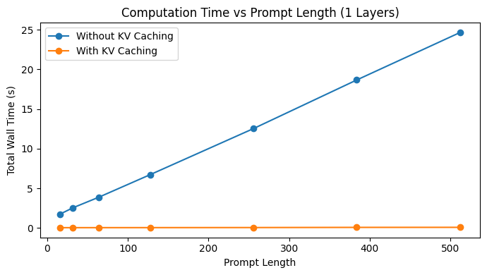
Figure 4: Comparison between computation time vs Prompt Length
Computational Cost Comparison:
This table reiterates the efficiency gain from KV caching across different sequence lengths.
| Sequence Length | Cache(MB) | With Cache(s) | Without Cache(s) | Speedup |
|---|---|---|---|---|
| 16 | 0.13 | 0.047 | 1.765 | 37.80x |
| 32 | 0.16 | 0.048 | 2.560 | 52.94x |
| 64 | 0.22 | 0.051 | 3.890 | 76.84x |
| 128 | 0.35 | 0.054 | 6.745 | 125.44x |
| 256 | 0.60 | 0.062 | 12.545 | 200.85x |
| 384 | 0.85 | 0.083 | 18.669 | 224.15x |
| 512 | 1.10 | 0.090 | 24.643 | 274.18x |
Number of Layers scaling:
To observe the scaling behavior with model depth, I have fixed the prompt length and varied the number of layers.
| Layers | Cache(MB) | With KV Cache Wall Time (s) |
|---|---|---|
| 6 | 2.09 | 0.363 |
| 12 | 4.17 | 0.727 |
| 24 | 8.34 | 1.424 |
| 48 | 16.69 | 2.874 |
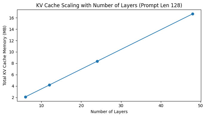
Figure 5: Comparison between computation time vs Prompt Length
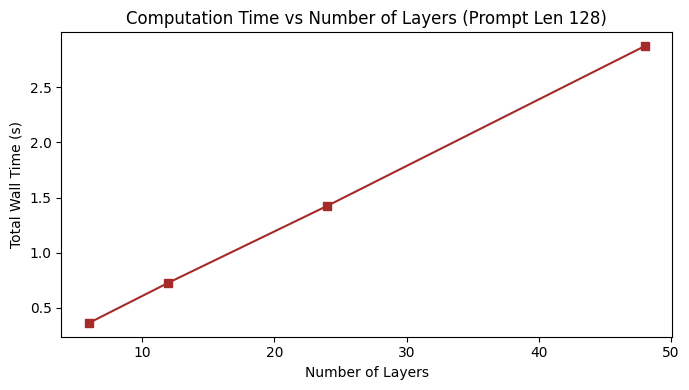
Figure 6: Comparison between computation time vs Prompt Length
While the toy network used in this example is intentionally minimalistic, the trends observed particularly regarding the effectiveness of KV caching will scale in similar patterns in larger architectures like those used in modern LLMs. Of course, the absolute memory and compute values will vary significantly depending on model dimensionality, depth, and implementation specifics.
The complete example code for benchmarking the performance is available at Demo Code.
Key Insights
The results from our analysis highlight several important trends in memory usage, performance gains, and trade-offs when employing KV caching in transformer-based models.
First, memory usage scales linearly with sequence length and complexity of network. As the prompt length increases, the size of the key-value (KV) cache grows proportionally. For larger models, especially those used in production-scale language applications, the cache size can surpass the memory footprint of the model parameters themselves, making memory management a critical consideration.
Second, the performance gains from caching are significant and increase with sequence length. In our tests, we observed speedups ranging from 10x to over 270x, with typical improvements falling in the 10–100x range for moderate length sequences. However, the benefits diminish for very short inputs, where the overhead of caching might outweigh the gains in execution time.
Lastly, there’s an inherent trade-off between memory and speed. While KV caching enables faster inference by avoiding redundant computations, it does so at the cost of increased memory usage, which can limit the effective batch size particularly on GPUs with constrained memory. This trade-off becomes especially relevant for real-time applications such as chatbots and code completion systems, where both latency and throughput are critical.
How do we optimize Key-value caching?
While key-value (KV) caching can significantly speed up inference in transformer models, it also introduces memory bottlenecks, especially at scale. To address these, several advanced optimization techniques have been proposed and are increasingly used in real-world systems. Below, I explore two such techniques inlcuding Grouped Query Attention (GQA) and Quantized KV Cache. But these are just the beginning, there are many more optimizations worth exploring in practice.
Tip 1 : Grouped Query Attention (GQA)
Grouped Query Attention reduces memory usage by sharing keys and values across multiple query heads. Instead of maintaining a separate key-value pair for each attention head, GQA uses fewer key-value heads (n_kv_heads) than query heads (n_heads). This technique is widely used in models like LLaMA and Mistral for efficient inferenceing.
Here’s the core implementation:
import torch
import torch.nn as nn

class GQAAttention(nn.Module):
    def __init__(self, dim, n_heads, n_kv_heads):
        super().__init__()
        assert n_heads % n_kv_heads == 0, "n_heads must be divisible by n_kv_heads"
        self.n_heads = n_heads
        self.n_kv_heads = n_kv_heads
        self.head_dim = dim // n_heads
        self.scale = self.head_dim ** -0.5

        self.q_proj = nn.Linear(dim, dim)
        self.k_proj = nn.Linear(dim, self.head_dim * n_kv_heads)
        self.v_proj = nn.Linear(dim, self.head_dim * n_kv_heads)
        self.out_proj = nn.Linear(dim, dim)

    def forward(self, x):
        B, T, C = x.size()
        q = self.q_proj(x).view(B, T, self.n_heads, self.head_dim)
        k = self.k_proj(x).view(B, T, self.n_kv_heads, self.head_dim)
        v = self.v_proj(x).view(B, T, self.n_kv_heads, self.head_dim)

        # Broadcast kv to match q heads
        k = k.repeat_interleave(self.n_heads // self.n_kv_heads, dim=2)
        v = v.repeat_interleave(self.n_heads // self.n_kv_heads, dim=2)

        attn_scores = (q @ k.transpose(-2, -1)) * self.scale
        attn_weights = torch.softmax(attn_scores, dim=-1)
        attn_output = attn_weights @ v

        out = attn_output.view(B, T, -1)
        return self.out_proj(out)
With this, we compare GQA against standard multi-head attention and observe the following:
=== Standard Multi-Head Attention ===
Standard Attention: Output shape: torch.Size([2, 128, 512]), Time: 0.2433s, CUDA Mem: 17.97 MB

=== Grouped Query Attention (GQA) ===
GQA Attention: Output shape: torch.Size([2, 128, 512]), Time: 0.0281s, CUDA Mem: 20.59 MB
The complete notebook is available at GQA Demo.
Tip 2 : Quantized KV Cache
As we’ve seen earlier, memory usage for KV caches scales linearly with both sequence length and the number of layers. So, quantizing the key and value tensors e.g., to int8 or int4 can dramatically reduce memory usage with a small trade-off in precision. Before using them in computation, the tensors are dequantized back to floating point. This technique is commonly used in real-time and resource-constrained settings, as it enables longer context lengths and/or bigger batch sizes.
Here’s a simplified PyTorch implementation of a quantized KV cache:
import torch
import time

class QuantizedKVCache:
    def __init__(self, n_heads, seq_len, head_dim, device="cpu"):
        self.n_heads = n_heads
        self.seq_len = seq_len
        self.head_dim = head_dim
        self.max_val = 127
        self.device = device
        self.scale_k = torch.ones(n_heads, 1, 1, device=device)
        self.scale_v = torch.ones(n_heads, 1, 1, device=device)
        self.cache_k = torch.zeros(n_heads, seq_len, head_dim, dtype=torch.int8, device=device)
        self.cache_v = torch.zeros(n_heads, seq_len, head_dim, dtype=torch.int8, device=device)
        self.cur_len = 0

    def append(self, k_new, v_new):
        n = k_new.size(1)
        self.scale_k = k_new.abs().amax(dim=(1,2), keepdim=True).clamp_min(1e-6)
        self.scale_v = v_new.abs().amax(dim=(1,2), keepdim=True).clamp_min(1e-6)
        qk = (k_new / self.scale_k * self.max_val).round().clamp(-self.max_val, self.max_val).to(torch.int8)
        qv = (v_new / self.scale_v * self.max_val).round().clamp(-self.max_val, self.max_val).to(torch.int8)
        self.cache_k[:, self.cur_len:self.cur_len+n] = qk
        self.cache_v[:, self.cur_len:self.cur_len+n] = qv
        self.cur_len += n

    def get(self):
        k = (self.cache_k[:, :self.cur_len].float() * self.scale_k / self.max_val)
        v = (self.cache_v[:, :self.cur_len].float() * self.scale_v / self.max_val)
        return k, v
And here’s the observed output when comparing quantized vs standard cache:
=== Standard (float32) KV Cache ===
Standard cache_k: 1048576 elements, 4 bytes/elem, 4.19 MB
Runtime: 0.0003s

=== Quantized (int8) KV Cache ===
Quantized cache_k: 1048576 elements, 1 bytes/elem, 1.05 MB
Runtime: 0.0701s

Quantization Error: mean(|orig - dequant|) for k: 0.008592, for v: 0.008716
The complete notebook is available at Quantized KV Demo.
Conclusion and Future Directions
Key-Value caching represents a fundamental breakthrough in transformer inference optimization, providing substantial performance improvements with manageable memory overhead. The mathematical analysis demonstrates clear scaling behaviours and trade-offs that inform deployment decisions.
Looking ahead, several promising research directions will likely transform how KV caching is implemented and utilized
- Advanced Cache Management:
Current KV caches typically use simple FIFO eviction when memory limits are reached. Future systems will implement adaptive policies that analyze attention patterns in real-time to identify which cached entries are most likely to be reused. e.g. a cache manager might preserve key-value pairs from tokens that consistently receive high attention weights across multiple layers, while aggressively evicting those from tokens with declining relevance. This could reduce cache misses at a greater efficiency compared to naive eviction strategies.
- Dynamic Sparsity:
Advanced systems will implement real-time pruning of KV caches based on attention score analysis. By monitoring which tokens consistently receive low attention weights, the system can dynamically remove their cached representations while maintaining output quality. This creates a self-optimizing cache that adapts to the specific attention patterns of each model and use case.
- Distributed Caching:
For large-scale deployments serving multiple users, distributed KV caching systems will emerge that can share cached computations across different inference servers. When User A asks about a topic, the resulting KV cache could be partially reused when User B asks a related question on a different server. This requires solving challenging problems around cache coherency, privacy preservation, and efficient cache lookup mechanisms across distributed systems.
The techniques presented here form the foundation for efficient large language model deployment, enabling real-time applications while managing computational resources effectively. As models continue to scale beyond current architectures, these optimizations become increasingly critical for making advanced AI systems practical and economically viable for widespread deployment.
Leave a Comment
Your email address will not be published. Required fields are marked *